Amp: a new measure of presortedness?

During the 80s, after decades of trying to find better sorting algorithms, some computer scientists started to formalize the concept of adaptive sorting, that is, sorting algorithms designed to take advantage of the existing order in a sequence of elements. This article is not about adaptive sorting algorithms.

This article is about the underlying notion of presortedness. When asked “what does it mean for a sequence to have existing order? How can we measure it?”, different authors came with different propositions:

The number of inversions in a sequence.
The distance between elements and their sorted position.
The number of groups of adjacent elements already in order.
The number of cycles of swaps needed to sort a sequence.
The size of the longest ascending subsequence.

It felt like a useful starting point, but once again a bit blurry and ad-hoc. Recognizing that issue, Heikki Mannila decided to formalize that a bit and published Measures of presortedness and optimal sorting algorithms in 1985, which brings a formal definition of measures of presortedness, describing the expected properties of functions meant to measure the existing order in a collection of elements—and also a formal definition of what an adaptive sort is, but once again this article isn’t about that.

Given two sequences $X$ and $Y$ of distinct elements, a measure of disorder $M$ is a function that satisfies the following properties:

If $X$ is sorted, then $M(X) = 0$

If $X$ and $Y$ are order isomorphic, then $M(X) = M(Y)$

If $X$ is a subsequence of $Y$, then $M(X) \le M(Y)$

If every element of $X$ is smaller than every element of $Y$, then $M(XY) \le M(X) + M(Y)$

‎$\forall a : M(\langle a \rangle X) \le \lvert X \rvert + M(X)$

We’re going to look back at those points more in-depth later, once we have introduced our own potential measure. Just a side note before moving on: I’m gonna keep using the term measure of presortedness for the rest of this article, though as you can see, those functions return 0 when the collection is already sorted, as such it would be more appropriate to call them measures of disorder—and lots of authors do actually call them that!—but old habits die hard, and I’m gonna stick to the words of Mannila.

Pairwise order of a sequence and its shadow

I’ve been toying with sorting-adjacent concepts for more than a decade now, and go on a tangent every now and then, exploring tiny tools under the length of sorting and combinations. A few days ago I went back to one of the simplest possible tools in the domain: a three-way comparator for two values:

\[comp(x, y)= \begin{cases} 1 & \text{ if } x \lt y\\ -1 & \text{ if } x \gt y\\ 0 & \text{otherwise} \end{cases}\]

Nothing ground-breaking so far, it’s similar to a negation of the sign function applied to the difference of two real numbers. Let’s apply it to all adjacent pairs of elements of a sequence of elements $X$:

Pairwise order of a sequence of elements: sequence 3, 4, 6, 6, 6, 7, 8, 6, 4 and the pairwise order 1, 1, 0, 0, 1, 1, -1, -1

Still fairly boring if I’m being honest. We will call that new sequence the pairwise order of the sequence for the rest of the article. Now let’s compute the prefix sum of that pairwise order:

Pairwise order shadow of a sequence of elements: sequence 3, 4, 6, 6, 6, 7, 8, 6, 4 and the pairwise order shadow 1, 2, 2, 2, 3, 3, 2, 1

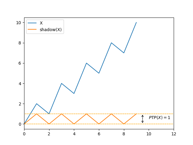
Now we get a cute result: a sequence of elements where the variations between adjacent elements follow those of the original sequence, except that the magnitude of those variations is always $0$ or $1$.

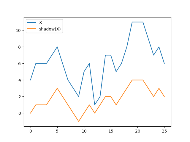
Line graph of a sequence of integers and its shadow

Okay, the previous statement is not exactly true: the original sequence has a size of $\lvert X \rvert$ while the prefix sum of the pairwise order has a size of $\lvert X \rvert - 1$. I constructed the plot above by prepending $0$ to the prefix sum, which leads to a new sequence of size $\lvert X \rvert$ whose variations between pairwise elements match those of the original sequence exactly. Interestingly, applying the same series of transformations on that $0$-pefixed prefix sum yields the same result again.

The plot above looks a bit like the original sequence has a midday shadow, so I decided to call the new structure the pairwise order shadow of the sequence, and will simply call it “shadow” for the rest of this article.

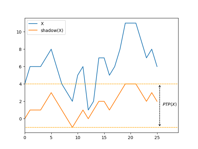
Peak-to-peak amplitude of a shadow

I started exploring that new mathematical object, and quickly wondered how much information about the order of the sequence was encoded into the peak-to-peak amplitude ($PTP$) of the shadow. The idea being that it could constitue a basis for a measure of presortedness.

Line graph of a sequence of integers and its shadow, which the peak-to-peak amplitude illustrated

A few simple observations can be made about $PTP$ rather intuitively:

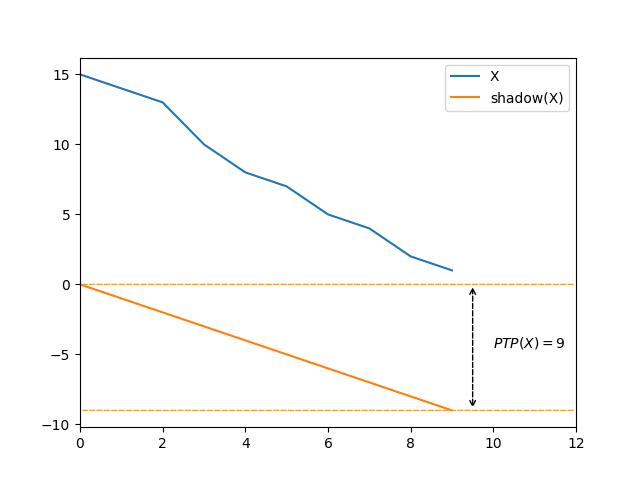
It is maximal when the sequence is strictly ascending or strictly descending, taking the value $\lvert X \rvert - 1$.
It is $0$ when all elements compare equal.
It is $1$ when the relative order of adjacent elements changes at each step.
It is at least as big as the longest ascending or descending run of the sequence.
It is direction-agnostic: the relative order of all adjacent elements could be flipped, $PTP$ would remain the same.

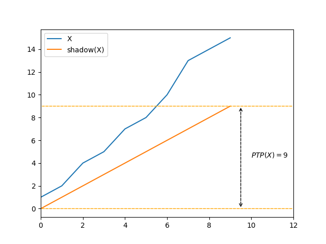
Strictly ascending sequence, PTP is maximal Strictly descending sequence, PTP is maximal Sequence oscillating at each step, PTP is minimal

If we ignore the issue of elements that compare equivalent, there is an intuition that a bigger $PTP$ means “more sorted”, and a lower $PTP$ means “less sorted”. Morever the direction-agnostic property is desirable, as it recognizes the pre-existing order in a strictly descending sequence. However, we can easily see shortcomings of the tool: in the last image graph above, it feels like the sequence is mostly ascending, but $PTP$ finds no order.

Here is another example of how $PTP$ fails to recognize some classes of pre-existing order:

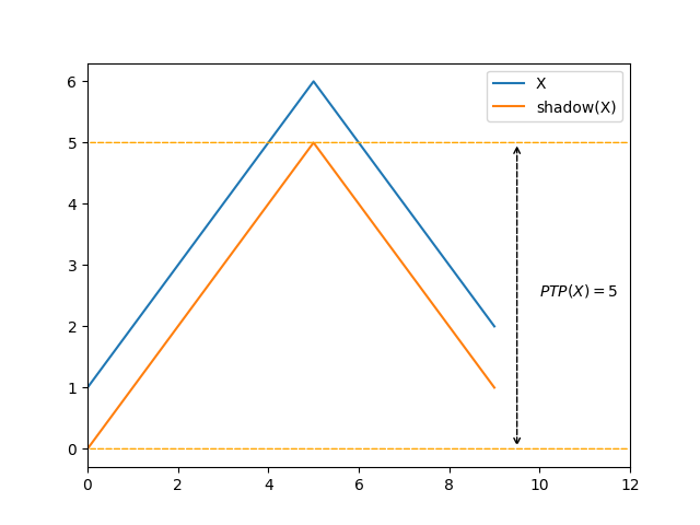
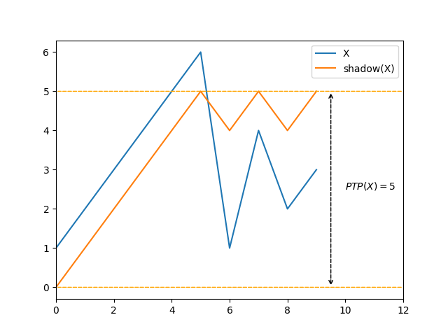
Sequence is an ascending run followed by a descending run, PTP is 5

The first pattern above is intuitively more ordered than the second one, however $PTP$ considers them both to bear the same amount of presortedness.

$Amp$: $PTP$ as a measure of presortedness

Despite its shortcomings, $PTP$ feels like a tool that can be used as a measure of presortedness: the greater it is, the more sorted the sequence should be, for some value of “sorted”. Feelings however are not enough, so we’re going to try our best to formally prove it. In order to do so, we need to go back to Mannila’s original criteria, and prove them one by one.

1. If $X$ is sorted, then $M(X) = 0$

Okay, we’re off to a bad start: $PTP(X)$ is maximal and equal to $\lvert X \rvert - 1$ when $X$ is sorted. Though that does not mean that we can’t use it as a measure of presortedness: we can just define the MOP based on $PTP$ as $\lvert X \rvert - PTP(X) - 1$. This gives us $0$ when $\lvert X \rvert$ is sorted, but also when $\lvert X \rvert$ is sorted in reverse order, which is a better basis for a MOP. For the rest of the article, we are going to call that new metric $Amp$.

Mannila’s original definition only considers sequences of distinct elements, but I am interested in real-life scenarios where elements can compare equivalent. The definition above gives $PTP(X) = 0$ and thus $Amp(X) = \lvert X \rvert - 1$ when $X$ is a sequence made of a single repeated element. We want such a sequence to be considered sorted and return $0$ instead. A simple workaround is to consider pairs of adjacent elements as ordered. Let’s call $N_{eq}$ the number of pairs of adjacent neighbours that compare equivalent, we get the following updated definition:

\[Amp(X) = \lvert X \rvert - PTP(X) - N_{eq}(X) - 1\]

We now have a more robust basis for a potential measure of presortedness, which at least satisfies criterion 1.

2. If $X$ and $Y$ are order isomorphic, then $M(X) = M(Y)$

The first step of our algorithm to compute $Amp(X)$ consists in stripping all information from $X$ except the relative order of adjacent elements. As such it is trivial to conclude that two order isomorphic sequences have the same pairwise order, the same shadow, and thus the same value for $PTP$ and for $Amp$.

3. If $SX$ is a subsequence of $X$, then $M(SX) \le M(X)$

The goal of that axiom is to make sure that a subsequence $SX$ of $X$ cannot have more absolute disorder than $X$ itself.

Proving that $Amp(SX) \le Amp(X)$ amounts to proving the following inequality:

\[\lvert SX \rvert - PTP(SX) - N_{eq}(SX) - 1 \le \lvert X \rvert - PTP(X) - N_{eq}(X) - 1\]

We can think of forming a subsequence of $X$ as removing elements anywhere from $X$, so we are going to analyze how the inequality above behaves when removing elements. The first observation we can make is that removing an elements only impacts the values of the comparisons between that element and its neighbours. As such, we can ignore the rest of the sequence for now and unroll the different scenarios when removing an element $n_i$ from $X$:

Elements	Pairwise order ($P_1$)	Pairwise order after removing $n_i$ ($P_2$)
$n_{i-1} = n_i = n_{i+1}$	$\langle 0, 0 \rangle$	$\langle 0 \rangle$
$n_{i-1} = n_i \lt n_{i+1}$	$\langle 0, 1 \rangle$	$\langle 1 \rangle$
$n_{i-1} = n_i \gt n_{i+1}$	$\langle 0, -1 \rangle$	$\langle -1 \rangle$
$n_{i-1} \lt n_i = n_{i+1}$	$\langle 1, 0 \rangle$	$\langle 1 \rangle$
$n_{i-1} \lt n_i \lt n_{i+1}$	$\langle 1, 1 \rangle$	$\langle 1 \rangle$
$n_{i-1} \lt n_i \gt n_{i+1}$	$\langle 1, -1 \rangle$	$\langle -1 \rangle \text{ or } \langle 0 \rangle \text{ or } \langle 1 \rangle$
$n_{i-1} \gt n_i = n_{i+1}$	$\langle -1, 0 \rangle$	$\langle -1 \rangle$
$n_{i-1} \gt n_i \lt n_{i+1}$	$\langle -1, 1 \rangle$	$\langle -1 \rangle \text{ or } \langle 0 \rangle \text{ or } \langle 1 \rangle$
$n_{i-1} \gt n_i \gt n_{i+1}$	$\langle -1, -1 \rangle$	$\langle -1 \rangle$

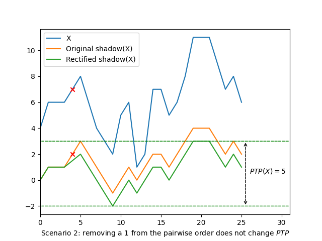
A first pattern arises from looking at the table above: when $P_1$ contains a $0$, $P_2$$ corresponds to $P_1$ with a $0$ removed. The interpretation here is that we are witnessing the transitivity of incomparability of the strict weak ordering. Crucially, it means that removing an element that compares equivalent to at least one of its neighbours only removes a $0$ from the pairwise order, which gives:

The $PTP$ does not change: removing a $0$ from the pairwise order only removes an element from the prefix sum based on it, without affecting the following numbers. As such the absolute maximum and minimum of the shadow remain the same, and therefore $PTP(SX) = PTP(X)$ in those scenarios.
The size of the sequence is reduced by $1$.
The number of pairs of neighbours that compare equivalent $N_{eq}$ is reduced by $1$.

In other words, given an element $E$ of $X$ than compares equivalent to at least one of its neighbours, we have:

\[\begin{aligned} Amp(X - \langle E \rangle) & = \lvert X - \langle E \rangle \rvert - PTP(X - \langle E \rangle) - N_{eq}(X - \langle E \rangle) - 1\\ & = (\lvert X \rvert - 1) - PTP(X) - (N_{eq}(X) - 1) - 1\\ & = \lvert X \rvert - PTP(X) - N_{eq}(X) - 1\\ & = Amp(X) \end{aligned}\]

This proves that removing any element from $X$ that compares equivalent to one of its neighbours does not change $Amp$ at all. We can extrapolate this result an consider that we can remove all $0$ elements from the pairwise order without affecting the $PTP$ nor $Amp$.

Line graph showing how removing zeros from the pairwise order does not change PTP

Consequently we can simplify the problem, and analyze the simpler inequality where no two neighbours compare equivalent ($N_{eq} = 0$):

\[\lvert SX \rvert - PTP(SX) - 1 \le \lvert X \rvert - PTP(X) - 1\]

Shuffle things around a bit, and we get this cute inequality to prove:

\[PTP(X) - PTP(SX) \le \lvert X \rvert - \lvert SX \rvert\]

We are gonna look again at the table from before, and analyze how this inequality behaves in the scenarios where the pairwise order does not contain any $0$:

Elements	Pairwise order ($P_1$)	Pairwise order after removing $n_i$ ($P_2$)
$n_{i-1} \lt n_i \lt n_{i+1}$	$\langle 1, 1 \rangle$	$\langle 1 \rangle$
$n_{i-1} \lt n_i \gt n_{i+1}$	$\langle 1, -1 \rangle$	$\langle -1 \rangle \text{ or } \langle 0 \rangle \text{ or } \langle 1 \rangle$
$n_{i-1} \gt n_i \lt n_{i+1}$	$\langle -1, 1 \rangle$	$\langle -1 \rangle \text{ or } \langle 0 \rangle \text{ or } \langle 1 \rangle$
$n_{i-1} \gt n_i \gt n_{i+1}$	$\langle -1, -1 \rangle$	$\langle -1 \rangle$

The first case removes $1$ from the pairwise order, which corresponds to removing one elements from the shadow, and subtracting $1$ from every subsequent element. Such a change can either increase $PTP$ by $1$, decrease it by $1$, or not change it at all.

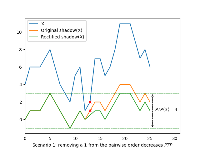
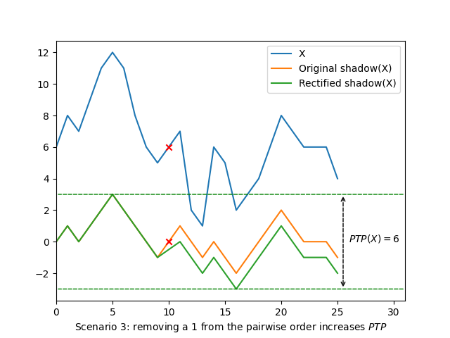
Line graph showing how removing one from the pairwise order can decrease PTP

$PTP(X) - PTP(SX)$ is minimal when $PTP(SX) = PTP(X) - 1$, in which case $PTP(X) - PTP(SX) = \lvert X \rvert - \lvert SX \rvert = 1$. Therefore the inequality we seek to prove is always true when removing an element $n_i$ such as $n_{i-1} \lt n_i \lt n_{i+1}$.

The case of removing an element $n_i$ such as $n_{i-1} \gt n_i \gt n_{i+1}$ corresponds to removing a $-1$ from the pairwise order, and is basically the same as removing a $1$ since it similarly results in $PTP$ changing by $0$, $1$ or $-1$.

The remaining cases are interesting: they both start with $\langle -1, 1 \rangle$ in some order in $P_1$, then have any of those removed to form $P_2$. $P_2 = \langle 1 \rangle$ and $P_2 = \langle -1 \rangle$ respectively correspond to removing $-1$ and $1$ from the pairwise order, which are scenarios we already analyzed above. The last remaining scenario to analyze is therefore when $P_2 = \langle 0 \rangle$: it might decrease $PTP$ by $1$ when the first removed element corresponds to an extremum of the shadow, in which case we get:

\[\begin{aligned} Amp(X - \langle E \rangle) & = \lvert X - \langle E \rangle \rvert - PTP(X - \langle E \rangle) - N_{eq}(X - \langle E \rangle) - 1\\ & = (\lvert X \rvert - 1) - (PTP(X) - 1) - (N_{eq}(X) + 1) - 1\\ & = \lvert X \rvert - PTP(X) - N_{eq}(X) - 2\\ & = Amp(X) - 1 \end{aligned}\]

With that last case covered, we just proved that removing an element from $X$ can never increase $Amp$. The logical extension of that result is that $Amp$ never increases, no matter how many elements we removed from it, in other words there exists no subsequence $SX$ of $X$ for which $Amp(SX) \gt Amp(X)$, which validates Mannila’s third criterion.

4. If every element of $X$ is smaller than every element of $Y$, then $M(XY) \le M(X) + M(Y)$

This is where our dream of proposing a new measure of presortedness gets shattered. Consider the following counter-example:

\[Amp(\langle 0, 1, 2, 3, 4 \rangle) = 0\] \[Amp(\langle 9, 8, 7, 6, 5 \rangle) = 0\] \[Amp(\langle 0, 1, 2, 3, 4, 9, 8, 7, 6, 5 \rangle) = 4\]

5. ‎$\forall a : M(\langle a \rangle X) \le \lvert X \rvert + M(X)$

That one is a almost trivial to prove: we know that for any sequence $X$, the highest possible value for $Amp(X)$ is $\lvert X \rvert - 1$. Therefore the highest possible value for $\langle x \rangle X$ is $\lvert \langle x \rangle X \rvert - 1 = \lvert X \rvert$.

Conclusion

To my greatest dismay, it appears that $Amp(X) = \lvert X \rvert - PTP(X) - N_{eq}(X) - 1$ is not a measure of presortedness by Mannila’s definition as it does not verify criterion 4. Does that mean that $Amp$ belongs into the trash pit of useless ideas? Maybe not: it does give some measure of the presortedness that pre-exists in a sequence, and can easily be computed in $O(n)$ time and $O(1)$ space with a simple linear scan, which is better than most existing measures of presortedness.

We will analyze other aspects of that new metric in subsequent articles, as well as its relation to existing measures of presortedness.

Elements	Pairwise order (\(P_1\))	Pairwise order after removing \(n_i\) (\(P_2\))
\(n_{i-1} = n_i = n_{i+1}\)	\(\langle 0, 0 \rangle\)	\(\langle 0 \rangle\)
\(n_{i-1} = n_i \lt n_{i+1}\)	\(\langle 0, 1 \rangle\)	\(\langle 1 \rangle\)
\(n_{i-1} = n_i \gt n_{i+1}\)	\(\langle 0, -1 \rangle\)	\(\langle -1 \rangle\)
\(n_{i-1} \lt n_i = n_{i+1}\)	\(\langle 1, 0 \rangle\)	\(\langle 1 \rangle\)
\(n_{i-1} \lt n_i \lt n_{i+1}\)	\(\langle 1, 1 \rangle\)	\(\langle 1 \rangle\)
\(n_{i-1} \lt n_i \gt n_{i+1}\)	\(\langle 1, -1 \rangle\)	\(\langle -1 \rangle \text{ or } \langle 0 \rangle \text{ or } \langle 1 \rangle\)
\(n_{i-1} \gt n_i = n_{i+1}\)	\(\langle -1, 0 \rangle\)	\(\langle -1 \rangle\)
\(n_{i-1} \gt n_i \lt n_{i+1}\)	\(\langle -1, 1 \rangle\)	\(\langle -1 \rangle \text{ or } \langle 0 \rangle \text{ or } \langle 1 \rangle\)
\(n_{i-1} \gt n_i \gt n_{i+1}\)	\(\langle -1, -1 \rangle\)	\(\langle -1 \rangle\)

Elements	Pairwise order (\(P_1\))	Pairwise order after removing \(n_i\) (\(P_2\))
\(n_{i-1} \lt n_i \lt n_{i+1}\)	\(\langle 1, 1 \rangle\)	\(\langle 1 \rangle\)
\(n_{i-1} \lt n_i \gt n_{i+1}\)	\(\langle 1, -1 \rangle\)	\(\langle -1 \rangle \text{ or } \langle 0 \rangle \text{ or } \langle 1 \rangle\)
\(n_{i-1} \gt n_i \lt n_{i+1}\)	\(\langle -1, 1 \rangle\)	\(\langle -1 \rangle \text{ or } \langle 0 \rangle \text{ or } \langle 1 \rangle\)
\(n_{i-1} \gt n_i \gt n_{i+1}\)	\(\langle -1, -1 \rangle\)	\(\langle -1 \rangle\)

Pairwise order of a sequence and its shadow

Peak-to-peak amplitude of a shadow

\(Amp\): \(PTP\) as a measure of presortedness

Conclusion