Amp and the partial ordering of measures of disorder, part 1

Shortly after computer scientists had proposed their first few measures of disorder, they started feeling an urge to show that their favourite measure was different from existing ones, and that they could actually come up with a single measure that was better than all the ones described by competitors.

Oozing manly energy, they reached for their best analytical tools, laid their most complicated data structures on paper — calling them “trivial” in an attempt to belittle their opponents and crush their will —, and started publishing paper upon paper in a glorious quest to scratch that competitive itch.

They naturally turned their attention to a few essential questions: how can we formally prove that two measures of disorder are equivalent? How can we can show that a measure of disorder is better than another one in the context of adaptive sorting?

Fearing day and night that someone else might publish the ultimate measure before they did, most turned to information gathering. Alas! No modern social network existed at the time, and they had to resort to simple mails to communicate, faking kindness and honest will to help in order to effectively spy on one another. Those prolific communications eventually turned to genuine bonding, all while precious mathematical insights were produced and published.

Maybe measures of disorder are the friends we made along the way?

At least that’s my headcanon.

In this article, I dive through the literature to understand how two measures of disorder can be compared. I then conjecture where \(\mathit{Amp}\) — which at this point has become the main protagonist of this blog — fits in the partial ordering of measures of disorder.

Comparing the values of measures of disorder

The simplest way to compare two measures of disorder is to compare the value they return for a given sequence. If a measure \(M_1\) returns a number that’s smaller than the one returned by another measure \(M_2\) for any sequence, then surely \(M_1\) has to be better than \(M_2\), right?

That reasoning feels sound when comparing some measures. For example:

• \(\mathit{SUS}\) is the number of increasing subsequences into which a sequence can be decomposed.
• \(\mathit{SMS}\) is the number of increasing or decreasing subsequences into which a sequence can be decomposed.

It makes intuitive sense that \(\mathit{SMS}\) always finds at most as many subsequences as \(\mathit{SUS}\), no matter the sequence they are applied to. A smaller number can then be interpreted as less absolute disorder. However this approach scales poorly, be it only because the codomains of different measures don’t always have the same range: for example \(\mathit{Runs}\) returns at most \(\lvert X \rvert - 1\) for a given sequence \(X\), while \(\mathit{Inv}\) can return as much as \(\frac{\lvert X \rvert(\lvert X \rvert - 1)}{2}\).

Recognizing that shortcoming, Estivill-Castro and Wood proposed the following definition in A New Measure of Presortedness:

Two measures of disorder \(M_1\) and \(M_2\) are equivalent iff there exists constraints \(c_1, c_2 > 0 \in \mathbb{N}\) such as \(c_1 M_1(X) \le M_2(X) \le c_2 M_1(X)\) for every sequence \(X\).

Using the results from a previous article, we can show that \(\mathit{Amp}\) is not equivalent to \(\mathit{Runs}\): indeed, \(\mathit{Runs}(X)\) returns \(\lvert X \rvert - 1\) when \(X\) is sorted in reverse order¹, where \(\mathit{Amp}\) returns \(0\) for such sequences. This makes it impossible to find a constant \(c_2 > 0\) such as \(\mathit{Runs}(X) \le c_2 \cdot \mathit{Amp}(X)\) for every sequence \(X\).

The linked article also proves that \(\mathit{Amp}(X) \le 2 \mathit{Runs}(X)\). Can we conclude that \(\mathit{Amp}\) is better than \(\mathit{Runs}\)? Not quite, though to understand why, we need to introduce another measure of presortedness: \(\mathit{Rem}\), the minimum number of elements to remove from a sequence to make it sorted.

In A Framework for Adaptive Sorting, Moffat and Pertersson show that \(\mathit{Runs}(X) \le \mathit{Rem}(X) + 1\) for any sequence \(X\)². The situation so is similar to the one we are trying to analyze with \(\mathit{Runs}\) and \(\mathit{Amp}\). They then give the following sequence to consider:

\[X = \langle 1, 2, 3, n, ..., n - \sqrt{n}, n, n - 1, n - 2, ..., n - \sqrt{n} + 1 \rangle\]

For such a sequence, we have \(\mathit{Runs}(X) = \sqrt{n}\) and \(\mathit{Rem}(X) = \sqrt{n} - 1\). For reasons we won’t discuss here, a \(\mathit{Runs}\)-optimal algorithm might spend \(\Theta(n \log{} n)\) time sorting \(X\), while a \(\mathit{Rem}\)-optimal algorithm is guaranteed to sort \(X\) in \(O(n)\) time³. The end result is that \(Runs\) is not “better” than \(Rem\) despite always returning a smaller value.

That shows that comparing the values of measures of disorder is not enough to tell whether one is better than the other. It is true even when the maximal value both measures can take is the same for any given input size.

Comparing measures in the context of adaptive sorting

The conclusion of the previous section carries a precious insight: we need to take a step back and forget about numbers. We need to reason in terms of the intuition that underlies measures of disorder: adaptive sorting.

Alistair Moffat proposes the following comparison and equivalence operators in Ranking measures of sortedness and sorting nearly sorted lists:

Let \(M_1\) and \(M_2\) be two measures of disorder:

• \(M_1\) is algorithmically finer than \(M_2\) (denoted \(M_1 \le_{\mathit{alg}} M_2\)) if and only if any \(M_1\)-optimal sorting algorithm is also \(M_2\)-optimal.
• \(M_1\) and \(M_2\) are algorithmically equivalent (denoted \(M_1 =_{\mathit{alg}} M_2\)) if and only if \(M_1 \le_{\mathit{alg}} M_2\) and \(M_2 \le_{\mathit{alg}} M_1\).

For practical reasons (rendering issues), the rest of this article uses the equivalent oprators \(\preceq\) and \(\equiv\), introduced by Jingsen Chen in Computing and Ranking Measures of Presortedness.

That definition is based on the practical function of measures of disorder: evaluating how much sorting algorithms can take advantage of the existing sortedness in a sequence.

Intuitively, it makes sense that a sorting algorithm that finds presortedness in both increasing and decreasing subsequences, finds presortedness in decreasing subsequences. In other words: \(\mathit{SMS} \preceq \mathit{SUS}\). Inversely \(\mathit{SUS}\) finds no presortedness in decreasing subsequences, so \(\mathit{SUS} \not \preceq \mathit{SMS}\) and \(\mathit{SMS} \not \equiv \mathit{SUS}\).

Formalizing that concept of optimality is non-trivial and out of scope for the current article. It will however be the topic of a subsequent article. In the meantime, we can look at the partial ordering of measures of disorder that’s obtained with the definition above:

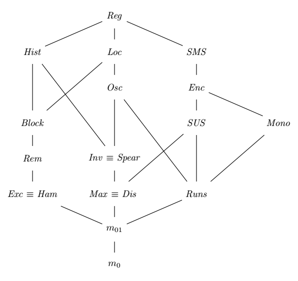
That graph is an extension of the one found in A Framework for Adaptive Sorting. Measures of disorder higher in the graph are algorithmically finer than those at the bottom, with links representing proven relationships between two measures. The “algorithmically finer” operator models a partial order, so transitivity can be assumed. It also means that some measures can be proven non-equivalent, without any having to be algorithmically finer than the other.

A few additional keys to read that graph:

• \(m_0\) is a measure of presortedness that always returns \(0\).
• \(m_{01}\) is a measure of presortedness that returns \(0\) when \(X\) is sorted and \(1\) otherwise.
• \(\mathit{Reg}\) is algorithmically finer than all other measures in the graph.

Applying to \(\mathit{Amp}\) what we learnt so far

I might not be exuding manly energy anymore, but I still want to know where \(\mathit{Amp}\) fits in the graph above. Let’s see what we learnt so far:

• We can prove equivalence of two measures of disorder by clamping the results of one between two multiplicative factors of the other.
• We can prove that a measure is not algorithmically finer than another by searching for patterns where only one of the measures finds sortedness.
• We don’t know yet how to prove that a measure is algorithmically finer than another.

This won’t be sufficient to find where \(\mathit{Amp}\) stands in the graph. We however might be able to prune just enough links to get a fairly good idea of where it should be.

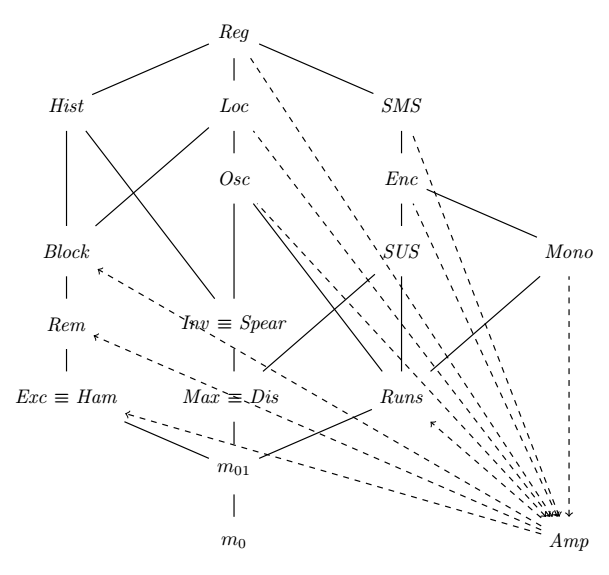
Let’s not assume any relationship to existing measures, and represent all hypotheses with dashed lines. We can’t rely on the “height” of \(\mathit{Amp}\) in the graph, because there’s too much we don’t know about it yet. As such, we represent a hypothesis such as “\(M_1\) is algorithmically finer than \(M_2\)” with an arrow from \(M_1\) to \(M_2\).

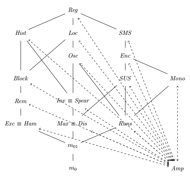
We are now going to apply what we learnt in order to untangle that spaghetti mess.

Descending runs

We proved earlier that \(\mathit{Runs}\) was not algorithmically finer than \(\mathit{Amp}\) by virtue of the latter finding sortedness in descending runs when the former does not. I actually actually consecrated a previous article to the topic of descending runs and presortedness, which tells us that \(\mathit{Block}\), \(\mathit{Dis}\), \(\mathit{Exc}\), \(\mathit{Ham}\), \(\mathit{Inv}\), \(\mathit{Max}\), \(\mathit{Rem}\), \(\mathit{Spear}\) and \(\mathit{SUS}\) find no sortedness in a descending run. It follows that none of those is algorithmically finer than \(\mathit{Amp}\). Transivity completes this list with \(\mathit{Hist}\).

We can reformulate that statement as follows, with \(M\) representing any of the aforementioned measures:

There is no constant \(c \in \mathbb{N}\) such as \(M(X) \le c \cdot \mathit{Amp}(X)\) for every sequence \(X\).

\(\mathit{Amp} \not \preceq \mathit{Mono}\)

\(\mathit{Mono}\) is the number of consecutive ascending and descending runs into which a sequence can be decomposed.

Let’s consider the following sequence, made of an ascending run of size \(\lceil \frac{\lvert X \rvert}{2} \rceil\) followed by a descending run of size \(\lfloor \frac{\lvert X \rvert}{2} \rfloor\):

\[X = \langle 0, 1, 3, ..., \frac{\lvert X \rvert}{2} - 1, \lvert X \rvert, \lvert X \rvert - 1, ..., \frac{\lvert X \rvert}{2} \rangle\]

For such a sequence, we have \(\mathit{Mono}(X) = 2\) and \(\mathit{Amp} = \lfloor \frac{\lvert X \rvert - 1}{2} \rfloor\):

There is no constant \(c \in \mathbb{N}\) such as \(Amp(X) \le c \cdot \mathit{Mono}(X)\) for every sequence \(X\).

In other words, \(\mathit{Amp}\) is not algorithmically finer than \(\mathit{Mono}\).

\(\mathit{Amp} \not \preceq \mathit{Max}\)

\(\mathit{Max}\) is the maximum distance an element of a sequence has to travel to reach its sorted position.

Let’s consider the following sequence, obtained by swapping pairs of elements in a sorted permutation:

\[X = \langle 1, 0, 3, 2, ..., n - 2, n - 3, n, n - 1 \rangle\]

For such a sequence, we have \(\mathit{Max}(X) = 1\) and \(\mathit{Amp} = \lvert X \rvert - 2\), which is the maximal value it can take.

There is no constant \(c \in \mathbb{N}\) such as \(Amp(X) \le c \cdot \mathit{Max}(X)\) for every sequence \(X\).

In other words, \(\mathit{Amp}\) is not algorithmically finer than \(\mathit{Max}\).

Transitively, this means that \(\mathit{Amp}\) cannot be algorithmically finer than \(\mathit{Dis}\), \(\mathit{Inv}\), \(\mathit{Spear}\), \(\mathit{Amp}\), \(\mathit{SUS}\), \(\mathit{Osc}\), \(\mathit{Enc}\), \(\mathit{Hist}\), \(\mathit{Loc}\), \(\mathit{SMS}\) nor \(\mathit{Reg}\).

Conclusion

Over the course of this article, we discovered that there’s more than meets the eye when it comes to comparing measures of disorders. A simple comparison of their results simply does not cut it. We need something more.

We could not prove that \(\mathit{Amp}\) was better than any other measure, neither could we prove that any other measure was better than \(\mathit{Amp}\). We could show however that some measures were not better than \(\mathit{Amp}\), and inversely that \(\mathit{Amp}\) was not better than some measures. Technically, that’s enough to prove the non-equivalence of \(\mathit{Amp}\) and a bunch of those measures.

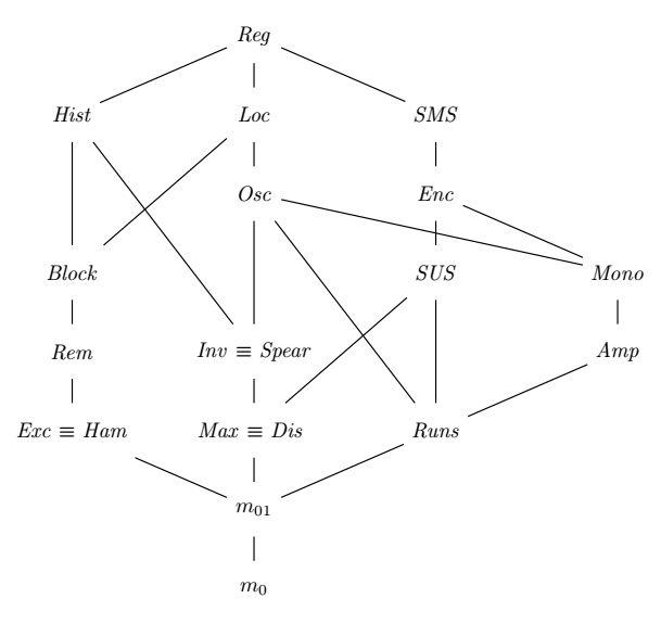
I can’t finish that article without a conjecture: my personal feeling is that \(\mathit{Mono} \preceq \mathit{Amp}\) and \(\mathit{Osc} \preceq \mathit{Mono}\)⁴. This means that the complete graph for the partial ordering would look like this:

In a future article, we will dig further and attempt to understand how to formally prove than a measure of disorder is better than another one.

Notes

1. A property that can be directly attributed to the symmetry of \(\mathit{Amp}\) over the input sequence. ↩

2. \(\mathit{Runs}\) counts the number of step-downs in a sequence (pairs of consecutive elements such as \(x_{i+1} > x_i\)). In any such pairs, at least one of the two elements cannot be part of the longest increasing subsequence of \(X\). It follows that \(\mathit{Runs} \le \mathit{Rem} + 1\). ↩

3. A result proven by Heikki Mannila in Measures of Presortedness and Optimal Sorting Algorithms. ↩

4. The place of \(Mono\) in the graph is actually also a conjecture. I applied similar reasoning that can be found in the original research section of cpp-sort’s documentation. ↩