Amp and the partial ordering of measures of disorder, part 2
In the first part of this series, we analyzed different techniques used to compare measures of disorder and to construct a partial order thereof. We then tried to apply that newfound knowledge to narrow down the place of \(\mathit{Amp}\) in the partial order.
That work remains unfinished as we haven’t yet learnt how to formally prove that a measure is “better” that another one. We instead settled on finding counter-examples to demonstrate that a measure of disorder is not better than another one.
Last time we mentioned the following comparison and equivalence operators proposed by Alistair Moffat in Ranking measures of sortedness and sorting nearly sorted lists1:
Let \(M_1\) and \(M_2\) be two measures of disorder:
- \(M_1\) is algorithmically finer than \(M_2\) (denoted \(M_1 \preceq M_2\)) if and only if any \(M_1\)-optimal sorting algorithm is also \(M_2\)-optimal.
- \(M_1\) and \(M_2\) are algorithmically equivalent (denoted \(M_1 \equiv M_2\)) if and only if \(M_1 \preceq M_2\) and \(M_2 \preceq M_1\).
However we never defined what it meant for a sorting algorithm to be \(M\)-optimal with regard to a measure of disorder \(M\). Today we’re digging deeper into what that notion of optimality means, and whether we can effectively use it to find the place of \(\mathit{Amp}\) in the partial order.
Measures of disorder and below-sets
The formal concept of adaptive sorting was pioneered by Heikki Mannila in his 1985 article Measures of presortedness and optimal sorting algorithms. After giving axioms describing what measures of presortedness are, Mannila defines the following function2:
Let \(M\) be a measure of presortedness and \(X\) a sequence of elements.
\(\mathit{below}_M(X) = \{ Y \vert Y \text{ is a permutation of } \langle 1, ..., \lvert X \rvert \rangle \text{ and } M(Y) \le M(X) \}\)
We say that \(\mathit{below}_M(X)\) is the below-set of the measure \(M\) for the sequence \(X\).
To get a better idea of what a below-set is, let’s analyze the below-set of \(Runs\)3 for the sequence \(\langle 4, 8, 1, 5 \rangle\):
| \(Y = \text{ permutation of } \langle 1, 2, 3, 4 \rangle\) | \(\mathit{Runs}(Y)\) |
|---|---|
| \(\langle 1, 2, 3, 4 \rangle\) | \(0\) |
| \(\langle 1, 2, 4, 3 \rangle\) | \(1\) |
| \(\langle 1, 3, 2, 4 \rangle\) | \(1\) |
| \(\langle 1, 3, 4, 2 \rangle\) | \(1\) |
| \(\langle 1, 4, 2, 3 \rangle\) | \(1\) |
| \(\langle 1, 4, 3, 2 \rangle\) | \(2\) |
| \(\langle 2, 1, 3, 4 \rangle\) | \(1\) |
| \(\langle 2, 1, 4, 3 \rangle\) | \(2\) |
| \(\langle 2, 3, 1, 4 \rangle\) | \(1\) |
| \(\langle 2, 3, 4, 1 \rangle\) | \(1\) |
| \(\langle 2, 4, 1, 3 \rangle\) | \(1\) |
| \(\langle 2, 4, 3, 1 \rangle\) | \(2\) |
| \(\langle 3, 1, 2, 4 \rangle\) | \(1\) |
| \(\langle 3, 1, 4, 2 \rangle\) | \(2\) |
| \(\langle 3, 2, 1, 4 \rangle\) | \(2\) |
| \(\langle 3, 2, 4, 1 \rangle\) | \(2\) |
| \(\langle 3, 4, 1, 2 \rangle\) | \(1\) |
| \(\langle 3, 4, 2, 1 \rangle\) | \(2\) |
| \(\langle 4, 1, 2, 3 \rangle\) | \(1\) |
| \(\langle 4, 1, 3, 2 \rangle\) | \(2\) |
| \(\langle 4, 2, 1, 3 \rangle\) | \(2\) |
| \(\langle 4, 2, 3, 1 \rangle\) | \(2\) |
| \(\langle 4, 3, 1, 2 \rangle\) | \(2\) |
| \(\langle 4, 3, 2, 1 \rangle\) | \(3\) |
The sequence \(\langle 4, 8, 1, 5 \rangle\) contains two runs, which means that \(\mathit{Runs}(\langle 4, 8, 1, 5 \rangle) = 1\). Its below-set consists of all sequences in the table above for which \(Runs\) returns \(0\) or \(1\), and its size is \(12\).
We have \(1 \le \mathit{below}_M(X) \le \lvert X \rvert !\) for any sequence \(X\) and any measure of disorder \(M\). That result holds because all the literature about measures of disorder only considers sequences of distinct elements, which means there exists at least one permutation of \({1, ..., \lvert X \rvert}\) which is order-isomorphic with \(X\).
I won’t mention sequences that contain equal elements in the rest of this article because no literature about those exists as far as I know, and I don’t have the required formal knowledge to fill in the blanks.
Finally, another property that makes below-sets interesting is that given two permutations \(X\) and \(Y\) of a same sequence and a measure of disorder \(M\), we have \(M(X) < M(Y) \implies \mathit{below}_M(X) < \mathit{below}_M(Y)\). All in all it gives us an operator to compare measures of disorder that satisfies two desirable properties:
- For a given sequence size, the returned values are in the same range regardless of the measure of disorder.
- The returned values always grow with disorder, no matter how it is measured.
Adaptive sorting
Mannila tackles the concept of adaptive sorting by defining what it means for a sorting algorithm to be adaptive with regard to a given measure of disorder. In his words:
Let \(M\) be a measure of presortedness, and \(S\) a sorting algorithm, which uses \(T_S(X)\) steps on input \(X\). We say that \(S\) is \(M\)-optimal (or optimal with respect to \(M\)), if for some \(c > 0\) we have for all \(X\):
\[T_S(X) \le c \cdot \max { \lvert X \rvert, \log \lvert \mathit{below}_M(X) \rvert }\]
Note: the notion of “steps” in the definition above can be understood as arbitrary constant-time operations, such as comparisons or elements swaps. For most of the analysis below, I am going to consider that they are comparisons, even though that’s technically an oversimplification.
To understand the definition above, we need to look at the two expressions passed to \(\max\). Let’s concentrate on \(\lvert \mathit{below}_M(X) \rvert\) first, since it is at the core of the concept of adaptive sorting: it is obtained by looking at the sorting problem through the lens of the decision tree model, a conceptual framework originally applied to sorting by Lester Ford & Selmer Johnson in their 1959 paper A Tournament Problem.
The decision tree model considers that we can perform comparisons of pairs of elements in a sequence \(X\) to uniquely identify an input permutation \(X\) among the \(\lvert X \rvert!\) possibilities. Let’s take \(X = \langle a, b, c \rangle\) and represent with a binary tree how we can use comparisons to uniquely identify each of its permutations.
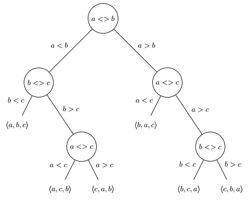
Assuming that all elements of \(X\) are distinct, we get a tree with \(\lvert X \rvert!\) leaves (here \(\lvert X \rvert! = 3! = 6\)). The direct corollary is that the minimal number of comparisons required to uniquely identify a sequence is at most the height \(h\) of that tree.
Any comparison sort implicitly follows such a comparison tree while operating, and always follows exactly one path to identify a given permutation4. However, information acquisition is generally not perfect: real-world algorithms perform comparisons to gather information they already had. A “perfect” comparison sort would be one that always collects the minimum amount of data needed to uniquely identify the permutation to sort, in which case the decision tree would approximate a perfect binary tree.
The height of a perfect binary tree of \(n\) elements is \(h = \log_2 n\), which here gives \(h = \log_2 2 \cdot (\lvert X \rvert!)\). Stirling’s approximation tells us that \(\log_2 \lvert X \rvert! \sim \lvert X \rvert \log_2 \lvert X \rvert\), which is where the \(O(n \log n)\) bound on comparison sorts originally comes from. Finding a practical algorithm that matches that lower bound is still an open problem to this day.
So… how does that relate to adaptive sorting?
As I understand it, an \(M\)-adaptive comparison sort is one where sequences for which \(M(X)\) is small appear as leaves higher in the decision tree, while those for which \(M(X)\) is bigger appear lower. It naturally follows that the algorithm performs less work to identify (sort) those “high” leaves than to identify the “low” ones. In such a model, \(\mathit{below}_M(X)\) can be seen as the permutations of \(X\) that are higher than \(X\) or at the same level in the decision tree of an \(M\)-optimal algorithm. The number of comparisons required to identify a sequence \(X\) in such a tree is thus related to \(\lvert \mathit{below}_M(X) \rvert\).
The second expression passed to \(\max\) in Mannila’s definition is a simple consideration: unless you have prior information, you need at least a linear number of comparisons to identify that said permutation is the sorted permutation.
Comparing measures of disorder with below-sets
Having a formal notion of what it means for a sorting algorithm to be \(M\)-optimal allows to inject it in Moffat’s comparison operators. That’s exactly what Jingsen Chen does in Computing and Ranking Measures of Presortedness:
Let \(\mathcal{M}\) be the set of all measures of presortedness and \(X\) be the sequence to be sorted. For \(M_1, M_2 \in \mathcal{M}\), we say that:
- \(M_1\) is superior to \(M_2\) (denoted \(M_1 \preceq M_2\)) if and only if there is some constant \(c > 0\) such that \(\lvert \mathit{below}_{M_1}(X) \rvert \le c \cdot \lvert \mathit{below}_{M_2}(X) \rvert\) for any sequence \(X\).
- \(M_1 \equiv M_2\) if \(M_1 \preceq M_2\) and \(M_2 \preceq M_1\).
That definition can be applied to compare the simplest measures of presortedness we have, namely \(m_0\) and \(m_{01}\):
\[\begin{aligned} m_0(X) &= 0\\ m_{01}(X) &= \begin{cases} 0 & \text{if } X \text{ is sorted }\\ 1 & \text{otherwise} \end{cases} \end{aligned}\]It logically follows that:
\[\begin{aligned} \lvert \mathit{below}_{m_0}(X) \rvert &= \lvert X \rvert !\\ \lvert \mathit{below}_{m_{01}}(X) \rvert &= \begin{cases} 1 & \text{if } X \text{ is sorted }\\ \lvert X \rvert ! & \text{otherwise} \end{cases} \end{aligned}\]We can conclude from it that \(\lvert \mathit{below}_{m_{01}}(X) \rvert \le \lvert \mathit{below}_{m_0}(X) \rvert\) for any sequence \(X\), so \(m_{01} \preceq m_0\). However there is no constant \(c > 0\) such as \(\lvert \mathit{below}_{m_0}(X) \rvert \le c \cdot \lvert \mathit{below}_{m_{01}}(X) \rvert\), so \(m_0 \not \preceq m_{01}\), and \(m_0 \not \equiv m_{01}\).
An interesting observation: \(\lvert \mathit{below}_{m_0}(X) \rvert = \lvert X \rvert ! \sim \lvert X \rvert \log_2 \lvert X \rvert\) for any sequence \(X\), which means that any \(O(n \log n)\) sorting algorithm is \(m_0\)-optimal.
That new definition is also enough to demonstrate the case from the first part of this series where \(\mathit{Runs} \not \preceq \mathit{Rem}\) despite having \(\mathit{Runs}(X) \le \mathit{Rem}(X) + 1\). Mannila proved the following bounds:
- \(\log \lvert \mathit{below}_{\mathit{Runs}}(X) \rvert = \Omega(\lvert X \rvert \log (1 + \mathit{Runs}(X)))\)
- \(\log \lvert \mathit{below}_{\mathit{Rem}}(X) \rvert = \Omega(\mathit{Rem}(X) \log (1 + \mathit{Rem}(X)))\)
As such there is no constant \(c > 0\) such that \(\lvert \mathit{below}_{\mathit{Runs}}(X) \rvert \le c \cdot \lvert \mathit{below}_{\mathit{Rem}}(X) \rvert\) for any sequence \(X\).
Computing the below-set of \(\mathit{Amp}\)
Armed with those new powerful tools, we’re eventually back to my original question: where does \(\mathit{Amp}\) fit within the partial order of measures of disorder?
We just have to compute \(\mathit{below}_{\mathit{Amp}}\) and compare it to that of other measures. It can’t be that hard… right?
Well, the truth is that all examples in the literature do either of two things to compute the below-set of a measure \(M\):
- Analyze existing \(M\)-optimal algorithms to understand how they work, and derive bounds from there,
- or attempt complicated demonstrations that involve combinatorics and factorials.
And that’s where it starts hurting: I don’t have a proven \(Amp\)-adaptive algorithm at hand, and my knowledge and instinct about properties of combinatorics and factorials are just anemic. If I am to attempt such a task, I first need some empirical data to draw conjectures and generalize from there.
Let’s start with a slightly different tool:
\[\mathit{equal}_M(X) = \{ Y \vert Y \text{ is a permutation of } \langle 1, ..., \lvert X \rvert \rangle \text{ and } M(Y) = M(X) \}\]You might recognize that it’s just the definition of a below-set but \(\le\) was replaced by an equal sign. I decided to compute \(\lvert \mathit{equal}_{\mathit{Amp}}(X) \rvert\) for sequences of \(0\) to \(10\) distinct elements, and to dump them into a table5:
| \(\lvert X \rvert\) / \(\lvert \mathit{equal}_{\mathit{Amp}} \rvert\) | 0 | 1 | 2 | 3 | 4 | 5 | 6 | 7 | 8 |
|---|---|---|---|---|---|---|---|---|---|
| 0 | 1 | ||||||||
| 1 | 1 | ||||||||
| 2 | 2 | ||||||||
| 3 | 2 | 4 | |||||||
| 4 | 2 | 12 | 10 | ||||||
| 5 | 2 | 16 | 70 | 32 | |||||
| 6 | 2 | 20 | 172 | 404 | 122 | ||||
| 7 | 2 | 24 | 334 | 1424 | 2712 | 544 | |||
| 8 | 2 | 28 | 632 | 3508 | 14408 | 18972 | 2770 | ||
| 9 | 2 | 32 | 1194 | 7984 | 47776 | 136948 | 153072 | 15872 | |
| 10 | 2 | 36 | 2276 | 17732 | 145274 | 558480 | 1515802 | 1288156 | 101042 |
We can see a few patterns emerging (disregarding the smaller sequences):
- The number of permutations for which \(\mathit{Amp}(X) = 0\) is always \(2\), which corresponds to the sorted and reverse sorted permutations.
- The number of permutations for which \(\mathit{Amp}(X) = 1\) is \(4(\lvert X \rvert - 1)\).
- The number of permutations for which \(\mathit{Amp}(X) = \lvert X \rvert - 2\), its maximum, corresponds to OEIS sequence A001250, the number of zigzag permutations of \(X\). Which makes sense because \(\mathit{Amp}\) reaches its worst case when the sign of the comparison between neighbors changes at each step.
After failing to understand André’s theorem, which computes the number of zigzag permutations of a given size, I decided that a general solution to compute \(\lvert \mathit{below}_{\mathit{Amp}} \rvert\) was definitely out of reach for my feeble mathematical skills.
Conclusion
For lack of better words, I am going to quote Jingsen Chen again:
For those measures with no optimal sorting algorithms adapting to them, the proof of the superiority between the measures might become quite difficult, since we may need to compute the exact sizes of the below-sets.
We sadly end this chapter without having been able to prove anything more about \(\mathit{Amp}\) and its place in the partial order. Though do not leave empty-handed either: we now have new powerful conceptual tools to understand disorder, as well as a few additional conjectures about the number of permutations for which \(\mathit{Amp}(X) = k\).
This is also not the end of the journey: I have more conjectures in store, and yet more angles to look at measures of disorder. Armed with enough knowledge and understanding of the appropriate mathematics, there could even be a third part of this series someday.
Until next time!
Notes
-
The operators proposed by Moffat are actually \(\le_{\mathit{alg}}\) and \(=_{\mathit{alg}}\). For practical reasons (rendering issues), we use the equivalent operators \(\preceq\) and \(\equiv\), introduced by Jingsen Chen in Computing and Ranking Measures of Presortedness. ↩
-
The original article also defines a more generic \(\mathit{below'}\) function, and uses a different syntax. ↩
-
\(Runs\) is defined as the number of ascending sequences of adjacent elements into which a sequence can be decomposed, minus \(1\). See one of my previous articles for more information about that measure of disorder. ↩
-
Unless randomness is influences decision-making in the algorithm, or more generally if the function is not pure. ↩
-
The equivalent table for \(\lvert \mathit{below}_{\mathit{Amp}} \rvert\) can be obtained by computing the prefix sum of each line, but I could not find any recognizable pattern in it. As a result, I decided not to include it in this blog post. ↩