Relationship between Amp and Mono

In this article, we analyze the relationship between the measure of disorder \(\mathit{Amp}\), which I introduced a while ago, and another measure of disorder: \(\mathit{Mono}\), the number of monotonic runs into which a sequence can be decomposed.

Identity of \(\mathit{Mono}\)

\(\mathit{Mono}\) is a measure of disorder originally described in [Sort Race][sort-race] by H. Zhang, B. Meng and Y. Liang:

Intuitively, if \(\mathit{Mono}(X) = k\), then \(X\) is the concatenation of \(k\) monotonic lists (either sorted or reversely sorted).

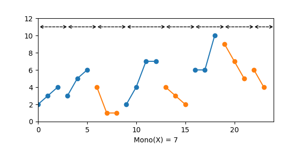
\(\mathit{Mono}\) is a natural extension of \(\mathit{Runs}\)¹ which seeks to find sortedness in both ascending and descending sequences. From a sorting point of view, it is useful to quantify the number operations performed by natural mergesorts that and merge detect monotonic runs.

A sorted sequence contains a single ascending run, so implementations of \(\mathit{Mono}\) might retrieve \(1\) to that number to obtain \(0\) for such a sequence (Mannila’s first axiom requires measures of presortedness to return \(0\) for sorted sequences). As a result we also get \(0\) for a single descending run, a symmetry which makes such an implementation unlikely to be a measure of presortedness². As a matter of fact, finding a counter-example showing that such an implementation violates Mannila’s 4th axiom is trivial:

If every element of \(X\) is smaller than every element of \(Y\), then \(M(XY) \le M(X) + M(Y)\)

Let’s consider two sequences \(X = \langle 0, 1, 2 \rangle\) and \(Y = \langle 5, 4, 3 \rangle\): we have \(\mathit{Mono}(X) = 0\) and \(\mathit{Mono}(Y) = 0\). However \(\mathit{Mono}(XY) = \mathit{Mono}(\langle 0, 1, 2, 5, 4, 3 \rangle) = 1\).

\(\mathit{Mono}\) can be computed with the following linear-time, constant-space algorithm:

1. Let \(n = 0\), and let the counter of mononic runs be \(0\).
2. Compare the elements \(X_n\) and \(X_{n+1}\) of the sequence:
   • If \(X_n < X_{n+1}\), compare the subsequent elements pairwise until a pair such as \(X_{n+k} > X_{n+k+1}\) is found.
   • If \(X_n > X_{n+1}\), compare the subsequent elements pairwise until a pair such as \(X_{n+k} < X_{n+k+1}\) is found.
   • If \(X_n = X_{n+1}\), restart at bullet 2 with \(n\) incremented by \(1\).
3. Add \(1\) to the counter of monotonic runs, repeat from bullet 2 with \(n = k+1\).
4. The result is the counter of monotonic runs minus \(1\).

The algorithm is almost as stupid as the description of \(\mathit{Mono}\) made it seem. And yet it is enough to see some patterns emerge:

• When two neighboring elements compare equal, they always belong to the same run³.
• A run contains at least two elements, except the last one which can be made of a single element.
• A direct corollary is that the maximum value \(\mathit{Mono}(X)\) can take is \(\lfloor \frac{\lvert X \rvert + 1}{2} \rfloor - 1\).
• That maximum value is notably attained for zigzag patterns, similar to \(\mathit{Amp}\), but also for other patterns.

Which brings us to the main topic of this article…

\(\mathit{Mono}\) and \(\mathit{Amp}\)

Previously, the only property I proved about the relationship between \(\mathit{Mono}\) and \(\mathit{Amp}\) was that \(\mathit{Amp} \not \preceq \mathit{Mono}\)⁴.

We additionally know that \(\mathit{Amp} \le 2 \mathit{Runs}\)¹, and it is easy enough to see that \(\mathit{Mono} \le \mathit{Runs}\) without an extensive proof⁵. However there is no transivity to exploit there, ergo nothing new to learn about the relationship between \(\mathit{Mono}\) and \(\mathit{Amp}\).

Without a simple mechanical process to apply and harvest new results, I decided to go back to gut feelings and reconsider the following conjecture:

\[\mathit{Mono} \le \mathit{Amp}\]

I had that simple inequality in mind for a while, and neither my brain not RapidCheck could find a counter-example to disprove it⁶.

The truth is, the previous article about the pairwise order was already an unspelled step in that direction: thanks to that preliminary work, we know that \(\mathit{Mono}(\mathit{Unique}(X)) = \mathit{Mono}(X)\) and that \(\mathit{Amp}(\mathit{Unique}(X)) = \mathit{Amp}(X)\). I figured that if I could simplify the problem to comparing the evolution of sequences of \(1\) and \(-1\), the conjecture would be easier to prove.

And yet, the definitions of \(\mathit{Mono}\) and \(\mathit{Amp}\) are just subtle enough that a direct proof felt out of reach. When comparing \(\mathit{Runs}\) and \(\mathit{Amp}\), I could reduce \(\mathit{Runs}\) to steps-down, and analyze the effect on those on \(\mathit{Amp}\). Neither \(\mathit{Amp}\) nor \(\mathit{Mono}\) trivially reduce to such a simple count of operations. Something more was needed.

Naps & Dreams to the rescue

The way I finally managed to tackle this problem is rather roundabout, and it’s high time to get personal with a far-fetched digression…

More than a decade as a professional software engineer has somehow left me mentally exhausted. I can barely work 5~6 hours a day before starting to get sleepy, to severely lose focus, at which point nothing I read makes sense anymore. Years of trying to fight that head-on did not lead to great results, and I had to resort to what long felt like a taboo: sleeping on my working hours.

Long naps tend to leave me dizzy and confused for longer than the duration of the nap, which does not work well either when it comes to working, so I settled on 15~20 minute ones⁷. My understanding is that I only reach early stages of light sleep, and avoid waking up from a deeper stage thereof: the transition seems to occur around the 30 minutes mark. I then get woken up by my alarm, wipe the drool off my pillow, and go back to work with a fresher mind and a renewed ability to focus. The end result is that I tend to be more productive — for some value of “productive” — than when I try to stay awake and focused without a nap.

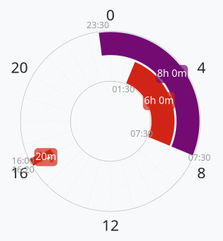
Trying to fall asleep midday, especially for such a short duration, is mostly of matter of habits and everyone has their own trick to make it work. I can’t really “empty my mind” — whatever that means — so I tend to let thoughts flow freely, without focusing too hard on any of them. Said thoughts often turn to mushy nonsense that only appears to mimick the concepts of mathematical logic, ridden with circular and tautological reasoning. It seems to be mostly seeded with whatever was on my mind at the time, so measures of disorder have made frequent appearances. The “discoveries” sometimes survive waking up, which is how I almost published an unrelated small article based on some absolutely wrong half-asleep insight a few months ago.

Another time, I woke up thinking I had found a simpler definition for \(\mathit{Mono}\) that would allow me to reason about it in simpler terms: the number of changes in the “direction” (ascending or descending) into which the values of the sequence grow.

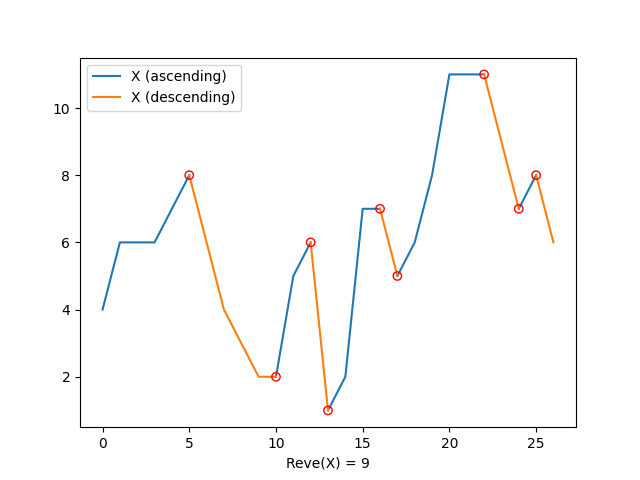
A cooler head qickly doused my hopes, and that eureka moment ended up feeling like something of a damp squib. Indeed, it is trivial to find sequences for which this new definition gives results different from \(\mathit{Mono}\):

• \(\mathit{Mono}(\langle 1, 3, 5, 2, 4 \rangle) = 1\) \(\)
• \(\mathit{DampSquib}(\langle 1, 3, 5, 2, 4 \rangle) = 2\) \(\)

\(\mathit{Reve}\), a new measure of disorder

Unwilling to entirely jettison the new toy my mushy brain had given me, I decided to treat it as a proper measure of disorder and analyze it further.

I gave it the name \(\mathit{Reve}\), partly because it counts “reversals” in the pairwise order, and partly because “rêve” is French for “dream” — a fitting name for a slumber artifact.

With such a simple definition, I quickly managed to identify a number of basic properties:

• The maximum value taken by \(\mathit{Reve}(X)\) is \(\lvert X \rvert - 2\) for a zigzag pattern.
• \(\mathit{Reve}(X)\) gathers all of its information by comparing adjacent elements of \(X\). It can therefore be defined in terms of the pairwise order of \(X\).
• If we consider that two equal neighbors in \(X\) never trigger a reversal, then it follows that \(\mathit{Reve}(\mathit{Unique}(X)) = \mathit{Reve}(X)\). Only the \(1\) and \(-1\) elements of the pairwise order are relevant to the analysis.
• A \(1\) followed by a \(-1\) in the pairwise order increases the disorder by \(1\), and so does a \(-1\) followed by a \(1\). It logically follows that \(\mathit{Reve}(\mathit{Reversed}(X)) = \mathit{Reve}(X)\)⁸.
• That last property is also a hint that, just like \(\mathit{Mono}\), \(\mathit{Reve}\) does not satisfy Mannila’s 4th axiom and is therefore not a measure of presortedness. Taking the same sequences as before, \(X = \langle 0, 1, 2 \rangle\) and \(Y = \langle 5, 4, 3 \rangle\), we indeed have \(\mathit{Reve}(X) = 0\) and \(\mathit{Reve}(Y) = 0\), but \(\mathit{Reve}(XY) = 1\).

Interestingly, \(\mathit{Reve}\) lends itself to a straightforward definition in terms of \(\mathit{Unique}\)⁹ and \(\mathit{Order}\):

\[\mathit{Reve}(X) = \lvert \mathit{Unique}(\mathit{Order}(\mathit{Unique}(X))) \rvert - 1\]

\(\mathit{Reve}\) and \(\mathit{Mono}\)

Whatever instinct I had while drowning my pillow in drool turned up to be close enough from \(\mathit{Mono}\) in terms of fundamental properties. I decided to have a closer look at the relationship between the two measures.

Since both can be defined in terms of the pairwise order, and both also satisfy the \(M(\mathit{Unique}(X)) = M(X)\) property, comparing them amounts to analyzing the effect of changes in a sequence of \(1\) and \(-1\).

• \(\mathit{Reve}\) is the simpler here: when two neighbors have different values, the disorder increases by \(1\). When two neighbors have the same value, the disorder does not increase.
• \(\mathit{Mono}\) is slightly more complicated: when two neighbors have different values, the disorder increases by \(1\) unless they are the first two elements of a new run.

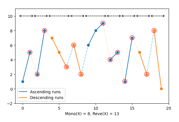
A window of \(4\) different elements is enough to analyze the difference between the two measures. Such a window has \(24\) possible permutations, but only \(8\) possible values for the pairwise order. Let’s unroll those \(8\) possibilities.

Pairwise order of \(\mathit{Unique}(X)\)	Example \(X\)	\(\mathit{Mono}(X)\)	\(\mathit{Reve}(X)\)
\(\langle 1, 1, 1 \rangle\)	\(\langle 0, 1, 2, 3 \rangle\)	\(0\)	\(0\)
\(\langle 1, 1, -1 \rangle\)	\(\langle 0, 1, 3, 2 \rangle\)	\(1\)	\(1\)
\(\langle 1, -1, 1 \rangle\)	\(\langle 0, 2, 1, 3 \rangle\)	\(1\)	\(2\)
\(\langle 1, -1, -1 \rangle\)	\(\langle 0, 3, 2, 1 \rangle\)	\(1\)	\(1\)
\(\langle -1, 1, 1 \rangle\)	\(\langle 1, 0, 2, 3 \rangle\)	\(1\)	\(1\)
\(\langle -1, 1, -1 \rangle\)	\(\langle 1, 0, 3, 2 \rangle\)	\(1\)	\(2\)
\(\langle -1, -1, 1 \rangle\)	\(\langle 3, 2, 0, 1 \rangle\)	\(1\)	\(1\)
\(\langle -1, -1, -1 \rangle\)	\(\langle 3, 2, 1, 0 \rangle\)	\(0\)	\(0\)

As we can see, the main difference between \(\mathit{Mono}\) and \(\mathit{Reve}\) is the scenario where there’s two changes in “direction” in a row: in such a case, the disorder increases by \(2\) for \(\mathit{Reve}\), but only by \(1\) for \(\mathit{Mono}\). Pushing that to the extreme case of a zigzag permutation, \(\mathit{Reve}\) finds twice as much disorder as \(\mathit{Mono}\).

That observation naturally leads to the following inequality for any sequence \(X\):

\[\mathit{Mono}(X) \le \mathit{Reve}(X) \le 2 \mathit{Mono}(X)\]

We covered that specific kind of inequality in a previous article, where we encountered the following definition¹⁰:

Two measures of disorder \(M_1\) and \(M_2\) are equivalent iff there exists constraints \(c_1, c_2 > 0 \in \mathbb{N}\) such as \(c_1 M_1(X) \le M_2(X) \le c_2 M_1(X)\) for every sequence \(X\).

Substituting \(M_1\) and \(M_2\) with \(\mathit{Mono}\) and \(\mathit{Reve}\) respectively, and picking \(c_1 = 1\) and \(c_2 = 2\), we can conclude that:

\[\mathit{Mono} \equiv \mathit{Reve}\]

That equivalence means that we can use \(\mathit{Reve}\) instead of \(\mathit{Mono}\) when analyzing their place in the partial order of measures of disorder. Additionally, it means that any sorting algorithm adaptive to one measure is also adaptive to the other. A valuable result in and of itself, considering that the definition of \(\mathit{Reve}\) is simpler to reason about than that of \(\mathit{Mono}\).

\(\mathit{Reve}\) and \(\mathit{Amp}\)

\(\mathit{Reve}\) also shares some similarities to \(\mathit{Amp}\), even though the two measures cannot be equivalent¹¹. The most interesting such similarity concerns the maximum disorder:

• For both measures, the maximum disorder of a sequence \(X\) is \(\lvert X \rvert - 2\).
• Both find maximum disorder in zigzag permutations.
• Computing the equal-set¹² of \(\mathit{Reve}\) for a small number of inputs shows that the number of permutations for which \(\mathit{Reve}\) finds maximum disorder is exactly equal to the number of zigzag permutations for that number of inputs. We found a similar result for \(\mathit{Amp}\) in a previous article.

The resemblance does not stop there: we showed that both measures can be defined in terms of the pairwise order and satisfy the \(M(\mathit{Unique}(X)) = M(X)\) property. Once again we can attempt to analyze how they relate by looking at how they are affected by changes in the pairwise order for sequences without equal neighbors.

We already know how \(\mathit{Reve}\) works, so all we have left to do is analyze how differing neighbors in the pairwise order affect \(\mathit{Amp}\). Let’s go back to the original definition of \(\mathit{Amp}\):

\[\mathit{Amp}(X) = \lvert X \rvert - \mathit{PTP}(X) - N_{\mathit{eq}}(X) - 1\]

Where:

• \(\lvert X \rvert\) is the number of elements in the sequence \(X\).
• \(\mathit{PTP}(X)\) is the peak-to-peak amplitude of \(X\), which corresponds to the prefix sum of the pairwise order of \(X\).
• \(N_{\mathit{eq}}(X)\) is the number of neighbors in \(X\) that compare equal.

We already showed that we can ignore equal neighbors when comparing \(\mathit{Reve}\) and \(\mathit{Amp}\), which leaves two observations:

• A \(1\) followed by a \(-1\) (or the other way around) in a prefix sum cancels itself: \(\mathit{PTP}(X)\) does not grow, and \(\lvert X \rvert - \mathit{PTP}(X)\) grows by \(1\).
• A \(1\) followed by a \(1\) (or a \(-1\) followed by a \(-1\)) in the pairwise order does not contribute to disorder in \(\mathit{Reve}\), but might contribute \(1\) to the disorder in the prefix sum of \(\mathit{Amp}\) depending on the rest of the sequence.

It follows that \(\mathit{Amp}(X)\) always finds at least as much disorder as \(\mathit{Reve}(X)\) for any sequence \(X\). Combining that result with that of the previous section, we get:

\[\mathit{Mono}(X) \le \mathit{Reve}(X) \le \mathit{Amp}(X)\]

And that transitively proves the conjecture from the beginning of this article.

Conclusion

When my knowledge of formal methods failed me.

When my skillset proved insufficient to tackle the problem I set out to solve.

When my will and motivation started to falter.

A light shone at the end of the drooly nap.

I woke up, dazed, yet dragging behind me The Intuition.

The one reformulation that would make sense of it all.

And it was incorrect.

Fuck.

This new chapter in the analysis of \(\mathit{Amp}\) started with a conjecture, a sheer instinct. I tried to convince myself that it was correct through tinkering, in a deeply empirical fashion. I somehow advanced further by reconsidering wrong results I had quite literally dreamt of, and managed to turn that into a new useful tool. And to finish it off… well, back to thinking formally until it all seems to click.

And I think that’s beautiful!

Had I been skilled enough to compare the behaviour of \(\mathit{Amp}\) and \(\mathit{Mono}\) directly, I might have been able to prove my original conjecture without having to introduce \(\mathit{Reve}\). But I’m very happy I was unable to do so! Thanks to that, I end up with a new measure of disorder which is at the same time equivalent to \(\mathit{Mono}\), but also much simpler to define and reason about. For all I know it might be a key that I can use to prove more relationships in the future.

Besides, the whole process of managing to find a new intermediary measure felt incredibly satisfying. It reminded me of how mathematics exercises chain questions that have you demonstrate smaller results, only to use them a few questions later to solve bigger problems that would otherwise be too difficult to solve at once. Being able to reproduce that on an open problem was amazing.

Sadly, this is currently the end of the \(\mathit{Amp}\) saga: I still haven’t managed to prove where it stands in the partial order of measures of disorders, but I am out of leads to push the experiment further.

I need to go back to the drawing board, learn some more again, and… who knows? Maybe I will someday wake up with another incorrect conjecture, that will eventually lead me to new results <3

Notes

1. \(\mathit{Runs}\) is a measure of disorder which corresponds the number of ascending runs in a sequence minus \(1\). I already covered it some time ago in Relationship between Amp and Runs. ↩ ↩²

2. A result analyzed at length in How much disorder is there in a descending run?. ↩

3. The literature about measures of disorder generally only studies sequences of unique elements. As such, Zhang, Meng and Liang do not define how \(\mathit{Mono}\) behaves when it encouters equal neighbors. I unilaterally decided when first implementing probe::mono in cpp-sort to make it behave that way, but an alternative also made sense: to consider that equal neighbors belong to ascending runs but not to descending runs. The rationale is that reversing equal neighbors make a sorting algorithm unstable, so the measure would not be appropriate for those. This series of articles analyzes my original implementation however, so I am gonna stick to it for the time being. ↩

4. That result can be demonstrated with a simple example: given a sequence made of an ascending run followed by a descending run of size \(\frac{\lvert X \rvert}{2}\) each, \(\mathit{Mono}\) finds constant disorder (two runs), while \(\mathit{Amp}\) finds \(\frac{\lvert X \rvert - 1}{2}\), that is linear disorder. See Amp and the partial ordering of measures of disorder, part 1 for more information. ↩

5. The minimum number of monotonic runs in a sequence is smaller than or equal to the minimum number of ascending runs in a sequence by definition. An ascending run is a monotonic run. ↩

6. A note about my process here: I tend to add conjectures to cpp-sort’s test suite in the form of RapidCheck properties. Besides revealing potential implementation mistakes, I consider that “either the conjecture is true or the check will one day find a counter-example”. It might not be the most robust thing to add to a test suite, but it has historically had enough value to continue doing it. By the time I publish an article, the CI has typically run hundreds such checks, reinforcing my faith in the correctness of the conjecture. ↩

7. My sleep schedule, despite not being strict, often follows the pattern of an Everyman E1 biphasic sleep schedule. ↩

8. \(\mathit{Reversed}\) returns a sequence corresponding to the C++ algorithm std::reverse applied to the input sequence. ↩

9. \(\mathit{Unique}\) is akin to the C++ algorithm std::unique, which reduces groups of equal neighbors to a single element. See Pairwise order of a sequence of elements for more information. ↩

10. That definition was proposed by Estivill-Castro and Wood in A New Measure of Presortedness. ↩

11. We showed earlier that \(\mathit{Amp} \not \preceq \mathit{Mono}\) and that \(\mathit{Mono} \equiv \mathit{Reve}\). If \(\mathit{Amp} \equiv \mathit{Reve}\) then we would have \(\mathit{Amp} \equiv \mathit{Mono}\), which is possible iff \(\mathit{Amp} \preceq \mathit{Mono}\) and \(\mathit{Mono} \preceq \mathit{Amp}\), in direct contradiction with the first statement. ↩

12. \(\mathit{equal}_M(X) = \{ Y \vert Y \text{ is a permutation of } \langle 1, ..., \lvert X \rvert \rangle \text{ and } M(Y) = M(X) \}\). This tool is introduced by Mannila in Measures of presortedness and optimal sorting algorithms, along with the notion of below-set, the preferred tool to compare measures of disorder. See Amp and the partial ordering of measures of disorder, part 2 for more information. ↩