Relationships between Osc, Mono and Reve
It might be the end of this series for now, at least in the way I so far approached analysis of measures of disorder. I do plan to pursue work on the topic, albeit with new tools and new angles. It will require some learning though, and I don’t know whether it will produce expected results, so it might take a while before I settle down and write another article.
Those are the words with which I ended the previous article1. It took a mere days for it to become a lie in the making, and here we are again, ready to look at measures of disorder with the same eye we did before.
Picking up the job where we left it, today we’re going to further refine the location of \(\mathit{Mono}\) in the partial ordering of measures of disorder.
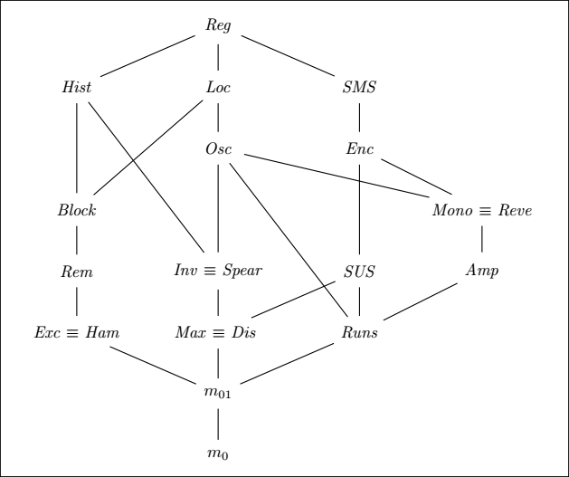
The last time, we left the picture above half-drawn, with the following conjectures left to prove:
- \(\mathit{Mono} \preceq \mathit{Amp}\)
- \(\mathit{Osc} \preceq \mathit{Mono}\) and \(\mathit{Mono} \not \preceq \mathit{Osc}\)
- \(\mathit{Loc} \preceq \mathit{Mono}\) and \(\mathit{Mono} \not \preceq \mathit{Loc}\), if the previous conjectures do not hold
We are gonna go one step up that ladder and look at the relationship between \(\mathit{Mono}\) and \(\mathit{Osc}\), a measure of disorder originally introduced by Christos Levcopoulos and Ola Petersson in Heapsort—Adapted for Presorted Files.
\(\mathit{Osc}\), the number of oscillations of a sequence
Let \(X = \langle x_1, ... x_{\lvert X \rvert} \rangle\) be a sequence of distinct elements. We define \(\mathit{Cross}(x_i)\) as follows:
\[\mathit{Cross}(x_i) = \{ j \vert 1 \le j < \lvert X \rvert \text{ and } \min{x_j, x_{j+1}} < x_i < \max{x_j, x_{j+1}} \}\]In the picture below, \(\mathit{Cross}(x_5)(\langle 6, 3, 9, 8, 4, 7, 1, 10 \rangle) = \langle 1, 3, 6 \rangle\):

The size of \(\mathit{Cross}(x_i)\) corresponds to the number of intersections between \(y = x_i\) and line segments joining direct neighbors of \(X\). We define \(\mathit{Osc}\) at the sum of those intersections:
\[\mathit{Osc}(X) = \sum_{i=1}^{\lvert X \rvert} \lvert \mathit{Cross}(x_i) \rvert\]A few properties of \(\mathit{Osc}\) qickly arise:
- It equals \(0\) for an ascending or descending sequence.
- It is perfectly symmetric over the input sequence2.
- It grows quadratically with disorder.
The actual maximum it reaches is \(\frac{\lvert X \rvert(\lvert X \rvert - 2)}{2}\) when \(\lvert X \rvert\) is even, and \(\frac{\lvert X \rvert(\lvert X \rvert - 2) - 1}{2}\) when \(\lvert X \rvert\) is odd.
\(\mathit{Osc}\) is called the oscillation measure because it appears to grow when the sequence oscillates between higher and lower elements.
\(\mathit{Osc}\) and \(\mathit{Runs}\)
A run is an ascending subsequence of neighboring elements in a sequence. It has been used as a measure of disorder for a long time due to its practicality in real-life scenarios. The measure of presortedness \(\mathit{Runs}(X)\) counts the number of runs in \(X\) and retrieves \(1\) from that number3, which means that it technically counts the steps-down in the sequence.
Levcopoulos and Petersson compare \(\mathit{Runs}\) to \(\mathit{Osc}\) as follows:
Clearly, for all \(i\), \(\mathit{Cross}(x_i)\) cannot contain more than two elements from each run […]. Furthermore, the run to which \(x_i\) belongs cannot contribute with more than one element to \(\mathit{Cross}(x_i)\).
The aforementioned “two elements” from each run are respectively:
- The element preceding the point where \(y = x_i\) “crosses” the run visually.
- The last element of the run, if \(y = x_i\) crosses the line segment between the last element of the run and the first element of the next run.
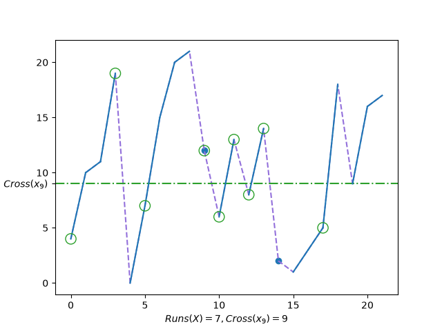
Keeping in mind that the numbers of runs in \(X\) is \(\mathit{Runs}(X) + 1\), we get the following inequality:
\[\begin{aligned} \mathit{Osc}(X) = \sum_{i=1}^{\lvert X \rvert} \lvert \mathit{Cross}(x_i) \rvert & \le \sum_{i=1}^{\lvert X \rvert} 2 \cdot (\mathit{Runs}(X) + 1) - 1\\ & = \sum_{i=1}^{\lvert X \rvert} 2 \cdot \mathit{Runs}(X) + 2 - 1\\ & = \sum_{i=1}^{\lvert X \rvert} 2 \cdot \mathit{Runs}(X) + 1\\ & = 2 \lvert X \rvert \cdot \mathit{Runs}(X) + \lvert X \rvert \end{aligned}\]Heapsort—Adapted for Presorted Files stops there, though the bound feels a bit weak, as there are other intuitive arguments to make: for example, the last run of \(X\) can contribute at most one element to \(\mathit{Cross}(x_i)\). If \(x_i\) is among the last run, then that run contributes zero element to \(\mathit{Cross}(x_i)\).
This consideration allows to remove one element from \(\mathit{Osc}(X)\) per \(\mathit{Cross}(x_i)\):
\[\mathit{Osc}(X) \le 2 \lvert X \rvert \cdot \mathit{Runs}(X)\]Can we do better still? Kind of, but that’s out of scope for the current article. I might revisit that inequality soon enough.
\(\mathit{Osc}\) and \(\mathit{Mono}\)
\(\mathit{Osc}\) is pretty much agnostic to the direction of a run, so the bound we found for \(\mathit{Runs}\) naturally also works for descending runs.
What about a combination thereof? I think you can easily convince yourself that the arguments from the previous section also apply to such a decomposition. It should be clear enough with a visual help:
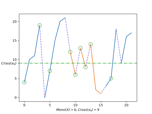
In other words:
\[\mathit{Osc} \le 2 \lvert X \rvert \cdot \mathit{Mono}(X)\]\(\mathit{Osc}\) and \(\mathit{Reve}\)
\(\mathit{Reve}\) is a measure that I introduced in a previous blog post4, where I showed that \(\mathit{Mono}(X) \le \mathit{Reve}(X) \le 2 \mathit{Mono}(X)\) for any sequence \(X\) — ergo, \(\mathit{Mono} \equiv \mathit{Reve}\).
\(\mathit{Reve}(X)\) corresponds to the number of changes in the “direction” (ascending or descending) into which the values of \(X\) grow.
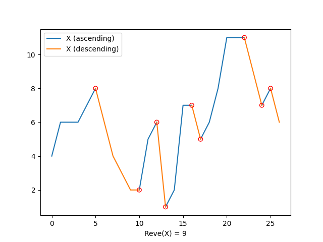
In many ways, \(\mathit{Reve}\) feels much closer from \(\mathit{Osc}\) than \(\mathit{Mono}\) ever did: instead of trying to find runs into which to decompose the sequence, it attempts to quantify its oscillation.
Its relationship to \(\mathit{Cross}\) is visually pretty obvious too:
- For a given element \(x_i\), there are at most \(\mathit{Reve}(X) + 1\) line segments that \(x_i\) might cross.
- \(x_i\) belongs to at least one of those segments — possibly two —, which therefore does not get added to \(\mathit{Cross}(x_i)\).
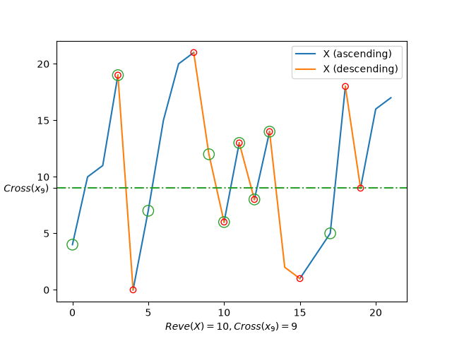
This leads to the following result:
\[\mathit{Osc}(X) = \sum_{i=1}^{\lvert X \rvert} \lvert \mathit{Cross}(x_i) \rvert \le \sum_{i=1}^{\lvert X \rvert} \mathit{Reve}(X) = \lvert X \rvert \cdot \mathit{Reve}(X)\]Which transitively gives:
\[\mathit{Osc}(X) \le \lvert X \rvert \cdot \mathit{Reve}(X) \le 2 \lvert X \rvert \cdot \mathit{Mono}(X) \le 2 \lvert X \rvert \cdot \mathit{Runs}(X)\]And that’s consistent with the bound we already found two sections ago. Sweet!
\(\mathit{Osc} \preceq \mathit{Mono}\)
Proving the superiority of \(\mathit{Osc}\) over \(\mathit{Mono}\) reuses the classification of measures of presortedness introduced by Chen and Carlsson in On Partitions and Presortedness of Sequences, which we already employed to prove \(\mathit{Enc} \preceq \mathit{Mono}\) in the previous post1.
Let \(C_A(M, X)\) be the minimum number of comparisons required for an \(M\)-optimal algorithm to sort \(X\). Let \(\mathcal{M}\) be the set of all measures of disorder, divided into disjoint subsets \(\mathcal{M}_i\) such as \(\mathcal{M} = \mathcal{M}_1 \cup \mathcal{M}_2 \cup \mathcal{M}_3 \cup \ldots\).
We define the following subsets of \(\mathcal{M}\):
- \(\mathcal{M}_1 = \{ M \in \mathcal{M} \vert C_A(M, X) = \Omega(\lvert X \rvert + \lvert X \rvert \log M(X)) \}\)
- \(\mathcal{M}_2 = \{ M \in \mathcal{M} \vert C_A(M, X) = \Omega(\lvert X \rvert + M(X) \log M(X)) \}\)
- \(\mathcal{M}_3 = \{ M \in \mathcal{M} \vert C_A(M, X) = \Omega(\lvert X \rvert + \lvert X \rvert \log \frac{M(X)}{\lvert X \rvert}) \}\)
For today’s measures, we know that:
- \(\mathit{Mono} \in \mathit{M_1}\), a result we already proved in the past1.
- \(\mathit{Osc} \in \mathit{M_3}\), which Levcopoulos and Pertersson obtain by showing that an \(\mathit{Osc}\)-optimal algorithm sorts a sequence \(X\) in \(\Omega(\lvert X \rvert + \lvert X \rvert \log \frac{\mathit{Osc}(X)}{\lvert X \rvert})\) comparisons.
In Computing and ranking measures of presortedness, Jingsen Chen gives the following theorem5:
Let \(a\) and \(b\) be positive constants. For any two measures \(M_1\) and \(M_2\) of presortedness and any sequence \(X\), if \(M_1 \in \mathcal{M}_3\) and \(M_2 \in \mathcal{M}_1\), and if \(M_1(X) \le a \cdot \lvert X \rvert \cdot M_2(X) + b\), then \(M_1 \preceq M_2\).
We showed earlier that \(\mathit{Osc}(X) \le 2 \lvert X \rvert \cdot \mathit{Mono}(X)\) for any sequence \(X\), which corresponds to Chen’s theorem above with \(a = 2\) and \(b = 0\).
Therefore \(\mathit{Osc} \preceq \mathit{Mono}~\blacksquare\)
Conclusion
While I still intend to look at measures of disorder through other yet undisclosed means, I am pretty happy to see that the intuitive approach I have used so far is still giving new results. Intuition is something I value a lot when trying to understand concepts.
I already have ideas for at least two subsequent articles, that immediately follow this one. Nothing new regarding \(\mathit{Amp}\)6 unfortunately, whose inferiority to \(\mathit{Mono}\) is the only piece left to solve the disorder puzzle as it so far stands. I might one day catch a glimpse of its shape during one of these fruitful naps.
Notes
-
See Mono in the partial ordering of measures of disorder. ↩ ↩2 ↩3
-
See Relationship between Amp and Runs for a longer rationale about how \(\mathit{Runs}\) is computed. ↩
-
\(\mathit{Osc}\) and \(\mathit{Mono}\) are not measures of presortedness according to Mannila’s definition due to violating axiom 4[^TODO], but they match Chen’s looser definition: If \(X \le Y\), then \(M(XY) \le M(X) + M(Y) + b\) for a constant positive integer \(b\). Both \(\mathit{Osc}\) and \(\mathit{Mono}\) have \(b = 1\). ↩
-
See Amp: a new measure of presortedness? for a definition of \(\mathit{Amp}\). ↩