Mono in the partial ordering of measures of disorder

In the previous article¹, I developed a new measure of disorder called \(\mathit{Reve}\) to make it easier to compare the values of \(\mathit{Amp}\)² and \(\mathit{Mono}\). I proved that the new measure was equivalent to \(\mathit{Mono}\), then conjectured that its simpler mathematical defnition would allow to more easily analyze relationships of \(\mathit{Mono}\) with other measures of disorder.

I wasn’t exactly wrong about the “analyze relationships of \(\mathit{Mono}\)” part: as a matter of fact it’s what this very blog post is about. \(\mathit{Reve}\), however, plays no part in those newfound results. Instead I’m going to rely on the tried-and-true mathematical trick of re-reading the literature and putting the pieces together.

In the following sections, we revisit the measures of disorder \(\mathit{Runs}\)³ and \(\mathit{Mono}\). In that process, we use variants of the classic mergesort algorithm to show through concrete examples how measures of disorder relate to adaptive sorting.

We then attempt to find the position of \(\mathit{Mono}\) in the partial ordering or measures of disorder, in a similar fashion to what we already for \(\mathit{Amp}\) in the past⁴⁵.

Top-down and bottom-up mergesorts

Top-down mergesort is a classic divide-and-conquer sorting algorithm, which works as follows:

1. If the sequence to sort has fewer than two elements, stop there.
2. Split the sequence to sort in half.
3. Recursively invoke mergesort on each of the two halves.
4. Merge the two now-sorted halves together.

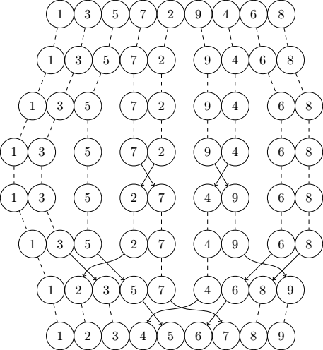
The algorithm performs \(O(n \log n)\) comparisons:

• “Splitting” the collection is a noop.
• Merging two sequences of sizes \(m\) and \(k\) requires \(O(m+k)\) comparisons.
• Merging all the subsequences pairwise at a given level of recursion requires \(O(n)\) comparisons.
• There are \(\log_2(n)\) levels of recursion⁶.

Bottom-up mergesort is a variant that performs similar work, but starts directly with sorting pairs of adjacent elements instead of repeatedly halving the collection until it reaches the level of pairs:

1. Sort pairs of adjacent elements in the sequence.
2. Merge adjacent pairs of elements to get sorted groups of \(4\) elements.
3. Merge adjacent groups of \(4\) elements to get sorted groups of \(8\) elements.
4. Repeat with groups twice as large each time, until the whole sequence is sorted.

When the number of elements in the sequence to sort is not a power of \(2\), then the last group of any level might be smaller than \(2^n\), in which case the algorithm either leaves it out or performs an unbalanced merge.

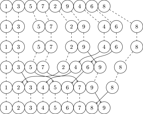
Both algorithms have the same complexity, and only differ in how they divide collections with an even number of elements at a given level. They perform exactly the same comparisons when the number of elements in the sequence to sort is a power of \(2\).

Natural mergesort

Natural mergesort is a variant of bottom-up mergesort that takes advantage of the existing order in a sequence: instead of using pairs of adjacent at its lowest level, it uses pairs of already sorted runs.

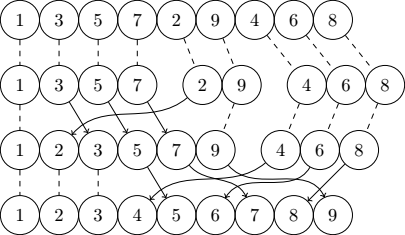
Instead of needing \(\log \lvert X \rvert\) levels of merge to sort a sequence \(X\), it only requires \(\log \mathit{Runs(\lvert X \rvert)}\) such levels.

The initial scan to gather runs requires \(X - 1\) comparisons, which leads to an overall complexity of \(O(\lvert X \rvert \log \mathit{Runs}(\lvert X \rvert))\). That’s virtually always better than \(O(\lvert X \rvert \log \lvert X \rvert)\) because \(\mathit{Runs}(X)\) is never greater than \(\lvert X \rvert\).

That result is an intuitive notion of what a \(\mathit{Runs}\)-adaptive sorting algorithm is. Mannila further proves⁷ that the \(O(\lvert X \rvert \log_2 \mathit{Runs}(\lvert X \rvert))\) bound is tight for \(\mathit{Runs}\): no sorting algorithm can do better in terms of the \(\mathit{Runs}\) measure alone. We therefore call natural mergesort \(\mathit{Runs}\)-optimal.

\(\mathit{Mono}\)-adaptive natural mergesort

\(\mathit{Mono}\) is a measure of disorder that corresponds to the minimal number of monotonic runs of into which a sequence can be decomposed. It was first introduced in Sort Race by H. Zhang, B. Meng and Y. Liang as follows:

Intuitively, if \(\mathit{Mono}(X) = k\), then \(X\) is the concatenation of \(k\) monotonic lists (either sorted or reversely sorted).

Computing \(\mathit{Mono}\) is a matter of doing the inverse operation of the concatenation described above: identifying the monotonic runs into which \(X\) can be decomposed, then retrieving \(1\) from their number to satisfy Mannila’s 1st axiom.

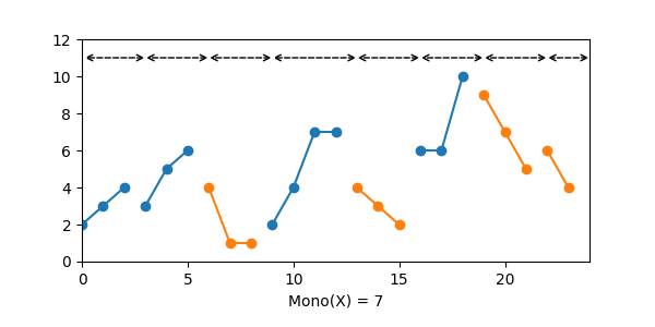
We can make natural mergesort \(\mathit{Mono}\)-adaptive by reversing the descending runs of that decomposition when we detect them, thereby turning them into ascending runs:

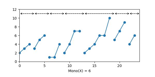
That operation takes linear time and turns a sequence \(X\) for which \(\mathit{Mono}(X) = k\) into a sequence \(Y\) for which \(\mathit{Runs}(Y) \le k\). It is pretty intuitive that this variant of natural mergesort runs in \(O(\lvert X \rvert \log \mathit{Mono}(X))\) time, making it a \(\mathit{Mono}\)-adaptive algorithm.

Is \(\mathit{Mono}\)-optimal though? Rather unsurprisingly, answering that question requires some additional work.

\(\mathit{Mono}\)-optimal natural mergesort

Computing the lower bound for a \(\mathit{Mono}\)-optimal algorithm would theoretically require computing the size of the corresponding below-set⁵, which “might become quite difficult” to paraphrase Jingsen Chen⁸.

Fortunately, Chen and Carlsson prove a fairly general result in On Partitions and Presortedness of Sequences, of which \(\mathit{Mono}\) is a mere special case. Quoting that paper:

Let \(\mathit{Spart}(\mathcal{T}, X)\) be the minimal size of a specific type \(\mathcal{T}\) of partitions [into which a sequence \(X\) of elements can be decomposed]. It is easy to show that \(\mathit{Spart}(\mathcal{T}, X)\) is a measure of presortedness […].

\(\mathit{Mono}\) clearly is a type of partition into which a sequence \(X\) can be decomposed. I am gonna assume that it is close enough from a measure of presortedness as far as \(\mathit{Spart}\) is concerned, despite violating Mannila’s 4th axiom of what constitutes such measures⁹.

Regardless, Chen and Carlsson then propose a general \(O(\lvert X \rvert \log \mathit{Spart}(\mathcal{T}, X))\) sorting algorithm, which consists in decomposing the sequence into partitions of type \(\mathcal{T}\), and using natural mergesort on those. The basic idea is exactly the same as the one we developed in the previous section.

However, they go one step further in their analysis and prove the following lower bound:

\(\Omega(\lvert X \rvert \log \mathit{Spart}(\mathcal{T}, X) + \lvert X \rvert)\) comparisons are necessary for any \(\mathit{Spart}\)-optimal algorithm to sort \(X\).

Considering that \(\mathit{Mono}(X) = \mathit{Spart}(\mathit{Mono}, X)\), it follows that the \(O(\lvert X \rvert \log \mathit{Mono}(X))\) bound we found for our natural mergesort variant is tight: our \(\mathit{Mono}\)-adaptive mergesort is also \(\mathit{Mono}\)-optimal.

\(\mathit{Mono}\) in the partial ordering or measures of disorder

All of the above was a rather long, but necessary prelude to the real topic of this article: finding the position of \(\mathit{Mono}\) in the partial ordering of measures of disorder.

It is an exercise that I already performed for \(\mathit{Amp}\) in the past⁴ — albeit inconclusively —, so I’m not going to repeat it all again. Readers can refer to the aforementioned blog post if they are unfamiliar with the methods employed.

As a reminder, here is the conjectured partial ordering:

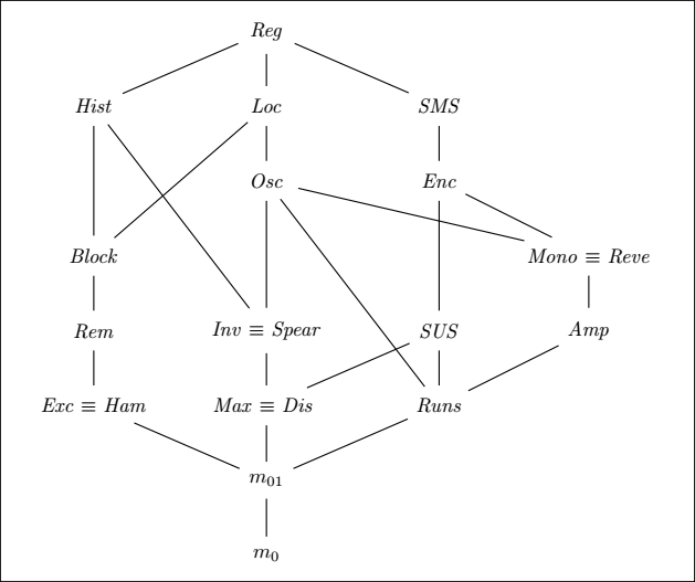
It is an extension of the ordering provided by Moffat and Petersson in A Framework for Adaptive Sorting, with \(\mathit{Amp}\) and \(\mathit{Mono}\) in the positions where I expect them to be. Crucially, I did not prove any of the visible links between those two measures and others: so far I only managed to prove that \(\mathit{Amp}\) was not superior to some other measures, and vice versa.

In the next subsections I am going to attempt to justify the place of \(\mathit{Mono}\) in the ordering above. If the process ever so slightly gives you a feeling of déjà-vu, it is because lots of the counter-examples that worked for \(\mathit{Amp}\) also work for \(\mathit{Mono}\).

Also, I shamelessly copy-pasted some of those subsections.

Descending runs

\(\mathit{Mono}\) considers a descending run to be sorted, which means that a measure that doesn’t find constant order in such a run cannot be superior to \(\mathit{Mono}\).

It immediately follows that \(\mathit{Block}\), \(\mathit{Dis}\), \(\mathit{Exc}\), \(\mathit{Ham}\), \(\mathit{Inv}\), \(\mathit{Max}\), \(\mathit{Rem}\), \(\mathit{Spear}\) and \(\mathit{SUS}\) are not superior to \(\mathit{Mono}\)⁹.

We can reformulate that statement as follows, with \(M\) representing any of the aforementioned measures:

There is no constant \(c \in \mathbb{N}\) such as \(M(X) \le c \cdot \mathit{Mono}(X)\) for every sequence \(X\).

\(\mathit{Mono} \not \preceq \mathit{Max}\)

\(\mathit{Max}\) is the maximum distance an element of a sequence has to travel to reach its sorted position.

Let’s consider the following sequence, obtained by swapping pairs of adjacent elements in a sorted permutation:

\[X = \langle 1, 0, 3, 2, ..., n - 2, n - 3, n, n - 1 \rangle\]

That sequence is a zigzag permutation, for which we have \(\mathit{Max}(X) = 1\) and \(\mathit{Mono} = \frac{\lvert X \rvert + 1}{2} - 1\), which is the maximal value it can take.

There is no constant \(c \in \mathbb{N}\) such as \(Mono(X) \le c \cdot \mathit{Max}(X)\) for every sequence \(X\).

In other words, \(\mathit{Mono}\) is not superior to \(\mathit{Max}\).

Transitively, this means that \(\mathit{Mono}\) is not superior to \(\mathit{Dis}\), \(\mathit{Enc}\), \(\mathit{Hist}\), \(\mathit{Inv}\), \(\mathit{Loc}\), \(\mathit{Osc}\), \(\mathit{Reg}\), \(\mathit{Spear}\), \(\mathit{SMS}\), nor \(\mathit{SUS}\).

\(\mathit{Amp} \not \preceq \mathit{Mono}\)

I already proved that result in a previous article⁴:

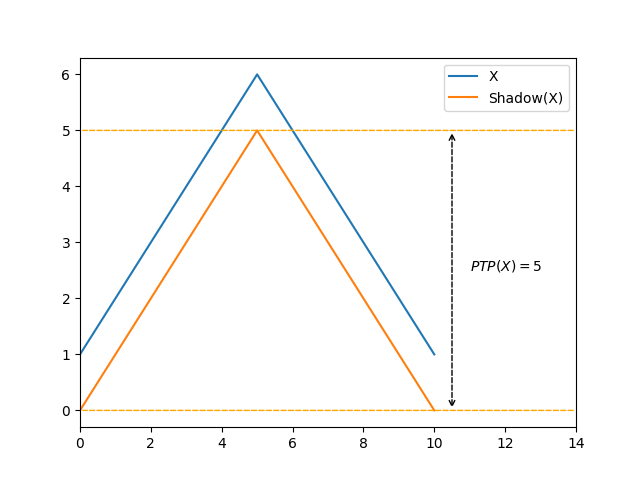
Let’s consider the following sequence, made of an ascending run of size \(\lceil \frac{\lvert X \rvert}{2} \rceil\) followed by a descending run of size \(\lfloor \frac{\lvert X \rvert}{2} \rfloor\):

\[X = \langle 0, 1, 3, ..., \frac{\lvert X \rvert}{2} - 1, \lvert X \rvert, \lvert X \rvert - 1, ..., \frac{\lvert X \rvert}{2} \rangle\]

For such a sequence, we have \(\mathit{Mono}(X) = 2\) and \(\mathit{Amp} = \lfloor \frac{\lvert X \rvert - 1}{2} \rfloor\):

There is no constant \(c \in \mathbb{N}\) such as \(Amp(X) \le c \cdot \mathit{Mono}(X)\) for every sequence \(X\).

In other words, \(\mathit{Amp}\) is not algorithmically finer than \(\mathit{Mono}\).

\(\mathit{Mono} \preceq \mathit{Runs}\)

We’re pretty much done repeating the exercise of showing that some measures are not superior to others. We can now move on to relations I had never been able to prove before: showing that some measures are superior to others.

On Partitions and Presortedness of Sequences provides the first necessary tool for the job, namely a simple classification of measures of disorder based on the complexity of adaptive sorting algorithms.

Let \(C_A(M, X)\) be the minimum number of comparisons required for an \(M\)-optimal algorithm to sort \(X\). Let \(\mathcal{M}\) be the set of all measures of disorder, divided into disjoint subsets \(\mathcal{M}_i\) such as \(\mathcal{M} = \mathcal{M}_1 \cup \mathcal{M}_2 \cup \mathcal{M}_3 \cup \ldots\).

We define the following subsets of \(\mathcal{M}\):

• ‎\(\mathcal{M}_1 = \{ M \in \mathcal{M} \vert C_A(M, X) = \Omega(\lvert X \rvert + \lvert X \rvert \log M(X)) \}\)
• ‎\(\mathcal{M}_2 = \{ M \in \mathcal{M} \vert C_A(M, X) = \Omega(\lvert X \rvert + M(X) \log M(X)) \}\)
• ‎\(\mathcal{M}_3 = \{ M \in \mathcal{M} \vert C_A(M, X) = \Omega(\lvert X \rvert + \lvert X \rvert \log \frac{M(X)}{\lvert X \rvert}) \}\)

As we saw earlier, \(\mathit{Runs}\) and \(\mathit{Mono}\), as well as all other measures \(M\) such as \(M(X) = \mathit{Spart}(M, X)\) belong to \(\mathcal{M}_1\).

In Computing and Ranking Measures of Presortedness, Chen restates the classification above in terms of the below-set of measures, then gives the following property:

Let \(a\) and \(b\) be positive constants. For any two measures \(M_1\) and \(M_2\) of presortedness and any sequence \(X\), if \(M_1\) and \(M_2\) belong to the same class \(\mathcal{M}_i (i = 1, 2, 3)\), and if \(M_1(X) \le a \cdot M_2(X) + b\), then \(M_1 \preceq M_2\).

We know that \(\mathit{Mono}(X) \le \mathit{Runs}(X)\) by virtue of an increasing run being a kind of monotonic run. We can therefore conclude that \(\mathit{Mono} \preceq \mathit{Runs}\)¹⁰.

\(\mathit{Enc} \preceq \mathit{Mono}\)

\(\mathit{Enc}(X)\) is the number of encroaching lists into which a sequence \(X\) can be decomposed. It was proposed by Steven S. Skiena in Encroaching Lists as a Measure of Presortedness, alongisde an \(\mathit{Enc}\)-adaptive algorithm called melsort (for Merge Encroaching Lists).

Melsort creates a collection of encroaching lists, then merges them together. Both phases require \(O(\lvert X \rvert \log \mathit{Enc}(X))\) comparisons, leading to a \(O(\lvert X \rvert \log \mathit{Enc}(X))\) sorting algorithm. Chen later showed that \(Enc(X) = \mathit{Spart}(Enc, X)\), thereby proving that melsort is \(\mathit{Enc}\)-optimal.

What are encroaching lists? They’re probably easier explained through their construction process from a sequence \(X\):

• Create an empty collection \(L\) of lists.
• Add a new list \(L_1\) to \(L\), which contains the first element of \(X\).
• For each other element \(X_i\) of \(X\):
  • If \(X_i\) is smaller than the first element of any list in \(L\), prepend \(X_i\) to the “oldest” such list.
  • If \(X_i\) is greater than the last element of any list in \(L\), append \(X_i\) to the “oldest” such list.
  • Otherwise, append a new list to \(L\) that contains \(X_i\).

That process can be seen as a “bidirectional” extension of the one used for [patience sorting][patience-sorting]. It creates a collection \(L\) of lists where:

• The first element of \(L_i\) is smaller than any element of \(L_{i+1}\).
• The last element of \(L_i\) is greater than any element of \(L_{i+1}\).

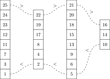
Here is an example of a decomposition into encroaching lists for the sequence \(\langle 23, 12, 11, 17, 7, 19, 3, 8, 13, 9, 15, 1, 22, 18, 14, 4, 2, 20, 6, 21, 5, 24, 16, 25, 10 \rangle\):

Skiena shows that \(\mathit{Enc}(X) \le \mathit{Runs}(X)\):

If \(X_i\) and \(X_{i+1}\) are part of the same run, they will end up on the same sublist \(l_j\). If not, \(X_i\) must have gone on an earlier sublist. The result follows since only one element per run can start a new sublist.

Thanks to the symmetry of encroaching lists, we can make a similar argument for descending runs. It logically follows that \(\mathit{Enc}(X) \le \mathit{Mono}(X)\) for any sequence \(X\).

Both \(\mathit{Enc}\) and \(\mathit{Mono}\) belong to \(\mathcal{M}_1\), which allows us to conclude that \(\mathit{Enc} \preceq \mathit{Mono}\).

Conclusion

Thanks to the transitive nature of the \(\preceq\) operator on measures of disorder, we can further refine the position of \(\mathit{Mono}\) in the partial ordering, leaving only a few conjectures to prove:

• ‎\(\mathit{Mono} \preceq \mathit{Amp}\)
• \(\mathit{Osc} \preceq \mathit{Mono}\) and \(\mathit{Mono} \not \preceq \mathit{Osc}\)
• \(\mathit{Loc} \preceq \mathit{Mono}\) and \(\mathit{Mono} \not \preceq \mathit{Loc}\), if the previous conjectures do not hold

I plan to publish new articles if I ever make advances on those topics, but the superior measures remain out of my analysis abilities to this day. Nevertheless, it’s interesting to see that most of the intuition-based conjectures I made in the past about the position of \(\mathit{Mono}\) do seem to hold.

It might be the end of this series for now, at least in the way I so far approached analysis of measures of dirsorder. I do plan to pursue work on the topic, albeit with new tools and new angles. It will require some learning though, and I don’t know whether it will produce expected results, so it might take a while before I settle down and write another article.

Until next time!

Notes

1. See Relationship between \(\mathit{Amp}\) and \(\mathit{Mono}\). ↩

2. See Amp: a new measure of presortedness?. ↩

3. See Relationship between \(\mathit{Amp}\) and \(\mathit{Runs}\). ↩

4. See \(\mathit{Amp}\) and the partial ordering of measures of disorder, part 1. ↩ ↩² ↩³

5. See \(\mathit{Amp}\) and the partial ordering of measures of disorder, part 2. ↩ ↩²

6. Halving a number until it reaches \(1\) is the very definition of a base \(2\) logarithm. ↩

7. See Measures of Presortedness and Optimal Sorting Algorithms by Heikki Mannila. I won’t attempt to explain the proof itself in this article, as it is fairly long, and lies beyond my understanding to this day. ↩

8. See Computing and Ranking Measures of Presortedness by Jingsen Chen. ↩

9. I provided a counter-example in a previous blog post¹, showing that \(\mathit{Mono}\) does not respect the 4th axiom. However, \(\mathit{Lads}\) suffers from the same issue, which does not prevent the paper from stating that \(\mathit{Lads} = \mathit{Spart}(\mathit{Lads}, X)\). That makes me believe that strict adherence to the 4th axiom is not a deal-breaker for \(\mathit{Spart}\). ↩ ↩²

10. Astute readers might have noticed that Chen’s definition specifically applies to measures of presortedness, yet we mentioned earlier that \(\mathit{Mono}\) was not a measure of presortedness due to not respecting Mannila’s 4th axiom. Fortunately, Chen’s paper works for a looser definition of measures of presortedness, where the 4th axiom reads If \(X \le Y\), then \(M(XY) \le M(X) + M(Y) + b\) for a constant positive integer \(b\). As it turns out, \(b = 1\) for \(\mathit{Mono}\), so we can reliably use the properties outlined by Chen. ↩